День 4 Летней школы Julia
Автор
Линейные уравнения
In [ ]:
gr()
Out[0]:
In [ ]:
A = rand( 4,4 ); b = rand( 4 );
A \ b
Out[0]:
In [ ]:
2 \ 4
Out[0]:
In [ ]:
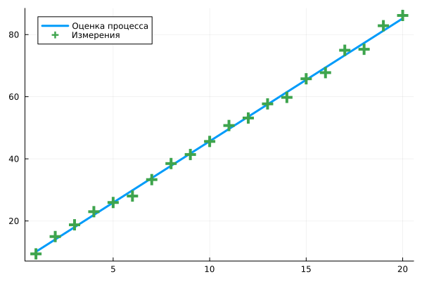
t = 1:20
y = 4t .+ 5 .+ 4*(rand( size(t)... ) .- 0.5)
a,b = [t ones(size(t)...)] \ y
Out[0]:
In [ ]:
plot( t, a*t .+ b, lw=3, label="Оценка процесса" )
scatter!( t, y, shape=:+, ms=8, msw=5, c=3, label="Измерения" )
Out[0]:
In [ ]:
]add HypothesisTests
In [ ]:
using HypothesisTests
In [ ]:
JarqueBeraTest( y .- (a*t .+ b) )
Out[0]:
In [ ]:
]add LinearSolve@2.39
In [ ]:
using LinearSolve
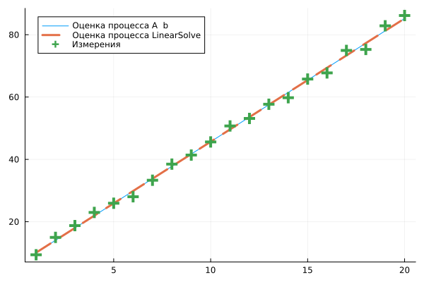
prob = LinearProblem( [t ones(t)], y )
linsolve = init( prob )
sol1 = solve( linsolve )
a2,b2 = sol1.u
Out[0]:
In [ ]:
plot( t, a*t .+ b, lw=1, label="Оценка процесса A \\ b" )
plot!( t, a2*t .+ b2, ls=:dash, lw=3, label="Оценка процесса LinearSolve" )
scatter!( t, y, shape=:+, ms=8, msw=5, c=3, label="Измерения" )
Out[0]:
In [ ]:
?LinearProblem()
Нелинейные уравнения
In [ ]:
# F(x) = 0
In [ ]:
]add Roots
In [ ]:
using Roots
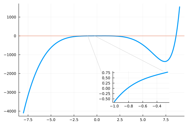
f1(x) = exp(x) - x^4
Out[0]:
In [ ]:
plot( [-8:0.1:9, -1:0.01:-0.25], [f1, f1], inset_subplots = bbox(0.6, 0.18, 0.3, 0.25, :bottom), leg=false, lw=3 );
hline!( [0] )
plot!( [-1, 1.7, 7.7, -0.25], [0, -3500, -2000, 0], c=:lightgray )
Out[0]:
In [ ]:
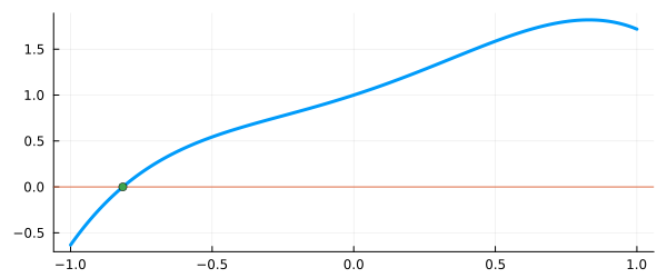
z = find_zero( f1, (-10,0) )
Out[0]:
In [ ]:
z = find_zero( f1, -10 )
Out[0]:
In [ ]:
plot( -1:0.01:1, f1, leg=false, lw=3 );
hline!( [0] )
scatter!( [z], [0], size=(600,250) )
Out[0]:
In [ ]:
z = find_zeros( f1, (-10,10) )
Out[0]:
In [ ]:
]add NonlinearSolve
In [ ]:
using NonlinearSolve
In [ ]:
function f2( dx, x, p )
    dx[1] = exp( x[1]) - x[1]^4
end
Out[0]:
In [ ]:
prob = NonlinearProblem( f2, [1.0] )
sol = solve( prob )
Out[0]:
In [ ]:
prob = NonlinearProblem( f2, [-10] )
sol = solve( prob )
Out[0]:
In [ ]:
using NonlinearSolve

function f3(du, u, p)
    x,y = u;
    du[1] = 2 - y - 3x;
    du[2] = x^2 + y^2 - 16;
end

prob = NonlinearProblem( f3, [0.0; 0.0] )
sol = solve( prob )
Out[0]:
In [ ]:
prob = NonlinearProblem( f3, [1.0; 1.0] )
sol2 = solve( prob )
Out[0]:
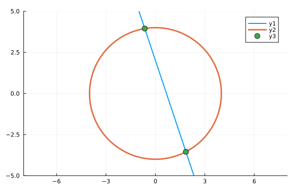
In [ ]:
]add ImplicitPlots
In [ ]:
using ImplicitPlots

fa(x,y) = 2 - y - 3x;
fb(x,y) = x^2 + y^2 - 16;

implicit_plot(fa; xlims=(-8,8), ylims=(-5,5), linecolor=1, lw=2)
implicit_plot!(fb; xlims=(-8,8), ylims=(-5,5), linecolor=2, lw=3)

x,y = sol.u
x2,y2 = sol2.u
scatter!( [x,x2], [y,y2], c=3, marker=(6) )
Out[0]:
Дифференциальные уравнения
In [ ]:
#]add DifferentialEquations
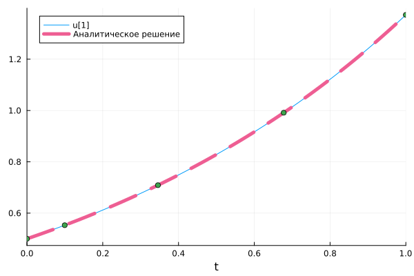
Решим вот такую задачу:
где и . Решение этого уравнения по мат.анализу: .
In [ ]:
using DifferentialEquations
f4(u,p,t) = 1.01*u
prob = ODEProblem( f4, 1/2, (0.0, 1.0))
sol = solve( prob )
Out[0]:
In [ ]:
sol(1)
Out[0]:
In [ ]:
plot(sol)
plot!( range(minimum(sol.t), maximum(sol.t),100), t->0.5*exp(1.01t), ls=:dash, lw=5, label="Аналитическое решение", c=7)
scatter!( sol.t, sol.u, label=false, c=3 )
Out[0]:
Задачи для изучения синтаксиса
Найти точку пересечения параболы y = x^2 и прямой y = 2x + 3.
In [ ]:
using NLsolve
function equations!(F, x)
    F[1] = x[1]^2 - x[2]    # y = x^2  -> x[1]^2 - x[2] = 0
    F[2] = 2*x[1] + 3 - x[2] # y = 2x+3 -> 2*x[1] + 3 - x[2] = 0
end
result = nlsolve(equations!, [0.0, 0.0]) # Начинаем поиск с точки (0,0)
println("Точка пересечения: x = ", result.zero[1], ", y = ", result.zero[2])
Найти максимум функции f(x) = -x^2 + 4x + 5 на интервале [0, 5] аналитически.
In [ ]:
using Symbolics
@variables x
f(x) = -x^2 + 4x + 5

# Находим производную
df = expand_derivatives(Differential(x)(f(x)))

# Решаем уравнение df/dx = 0
critical_point = symbolic_linear_solve(df ~ 0, x)

# Оцениваем значение функции в критической точке
f_max = f(critical_point)
println("Максимум функции: f($critical_point) = $f_max")