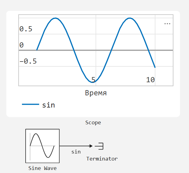
Scope

The unit is not recommended for use.

Display signals generated during simulation.

scope

Description

The Scope unit (Oscilloscope) displays signals in the time domain.

The oscilloscope is optimised for general time domain simulation.

Oscilloscope features:

Triggers - Set triggers to synchronise repeating signals and pause the display when events occur.
Cursor Measurements - measure signal values using vertical and horizontal cursors.
Signal Statistics - display the maximum, minimum, peak difference, mean, median and RMS of the selected signal.
Peak Finder - find peaks by showing the X-axis values where they occur.
Two Level Measurements - measure transitions, outliers, dips and cycles.

Volume Display Features:

Simulation Control - debug models from the Scope window using the Run, Step Forward, and Step Backward buttons on the toolbar.
Multiple signal - plot multiple signals on the same Y-axis (mapping) using multiple input ports.
Multiple y-axes (displays) - display multiple Y-axes. All Y-axes share a common time range over the X-axis.
Modify parameters - change oscilloscope parameter values before and during simulation.
Axis autoscaling - autoscale the axes during or at the end of the simulation. Fields are drawn at the top and bottom of the axes.
Display data after simulation - Scope data is saved during simulation. If the oscilloscope is closed at the beginning of the simulation, when you open the oscilloscope after the simulation, the oscilloscope displays the simulation results for the attached input signals.

If you have high sampling rates or long simulation times, you may experience memory or system performance problems because the oscilloscope stores data internally. To limit the amount of data stored for area visualisation, use the Limit data points to last property.

Limitations

Do not use area blocks in a library. If you place an area block inside a library block with a locked reference or in a locked library, an error will be displayed when you try to open the area window. To display internal data from a library block, add an output port to the library block, and then connect the port to the Scope block in your model.
When you step through the model, the scope is only updated when the scope block is started. This means that the time displayed in the status bar may not match the model time.
When connected to a DC signal, the oscilloscope block can display a single point.
The oscilloscope shows gaps in the display when the signal value is NaN.
When you visualise multiple signals based on frames in the oscilloscope, some signal samples with a frame size of 1 may not be displayed. To visualise these signals, move the signals with frame size 1 to a separate scope.
Oscilloscope displays have limitations in Rapid Accelerator mode.
When the Scope is in the ForEach subsystem, only the last index is displayed in the scope.

Ports

Input

Connect the signals you want to visualise. Up to 96 input ports can be used. The input signals can have the following characteristics:

Type - continuous (sample-based) or discrete (sample and frame-based).
Data Type - any data type that is supported.
Dimensionality - scalar, one-dimensional (vector), two-dimensional (matrix), or multidimensional (array). Display multiple channels in one signal depending on the dimensionality.

Input Limitations.

When the input represents a constant signal, the oscilloscope plots a single point.
The oscilloscope shows gaps on the display when the signal value is NaN.
When you visualise multiple signals based on frames in the oscilloscope, some sample signals with a frame size of 1 may not be displayed. To visualise these signals, move the signals with frame size 1 to a separate scope.

Bus Support

You can connect non-virtual bus and bus signal arrays to the oscilloscope. To display bus signals, use normal mode or accelerator simulation mode. The oscilloscope displays each bus element signal in the order in which the elements appear on the bus, from top to bottom. Nested bus elements are aligned.

To register non-virtual scope bus signals, set the Save format parameter to `Dataset'. You can use any save format to register virtual bus signals.

Data types: Float16, Float32, Float64, Int8, Int16, Int32, Int64, Int128, UInt8, UInt16, UInt32, UInt64, UInt128, Fixed.

Characteristics

Configuration properties

Main

Open at simulation start - specify when the Scope window opens
` disabled (by default for Scope)` | enabled

Select this checkbox to open the oscilloscope window when simulation starts.

Display the full path - display the block path in the title bar
off (By default) | on

Select this checkbox to display the path to the block in addition to the block name.

Number of input ports - number of input ports in the scope block
1 (by default) | an integer

Set the number of input ports in the Scope block as an integer. The maximum number of input ports is 96.

Layout - number and layout of displays
1 by 1 (by default) | `m by n' axis layout

Specify the number and arrangement of displays. The maximum layout is 16 rows by 16 columns.

If the number of displays is equal to the number of ports, signals from each port appear on separate displays. If the number of displays is less than the number of ports, signals from additional ports appear on the last display. For layouts with multiple columns and rows, ports are displayed down and then across.

Sample time - the interval between calculation steps
-1 (by default) | scalar

Specify the interval between calculation steps as a non-negative number. To inherit a calculation step, set this parameter to -1.

Input processing - signal processing method
Elements as channels (sample based) (by default) | Columns as channels (frame based)

Elements as channels (sample based) - the block processes each element as a unique sample.
Columns as channels (frame based) - the block processes signal values in a channel as a group of values from several time intervals. Frame processing is available only for discrete input signals.

Maximise axes - maximum size of charts
` disabled (by default)` | Auto | on

Auto - if the Header and Y-mark properties are not specified, maximise all charts.
On - maximise all plots. The values in the Header and Y-label are hidden.
disabled - do not maximise plots.

Time

Time span - length of X axis to be displayed
Auto (by default) | User defined | One frame period

Auto - difference between simulation start and end time.

The block calculates the start and end times of the time range using the Time display offset and Time span properties. For example, if Time display offset is set to 10 and Time span is set to 20, the range sets the time range from 10 to 30.
User defined - enter any value less than the total simulation time.
One frame period - use the frame period of the input signal for the Time Scope block. This parameter is available only if Input processing is set to Columns as channels (frame based).

Time span overrun action - display data outside the visible X axis
Wrap (By default) | Scroll

Specify how to display data outside the visible X-axis span.

The effect of this option can only be seen when building large models or small step sizes slowly.

Wrap - draw a full screen of data from left to right, clear the screen, and then restart drawing data from the left.
Scroll - move the data to the left as new data is drawn to the right. This mode is graphics intensive and can affect runtime performance.

Time units - X-axis units
None (by default) | Metric | Seconds

Metric - display of time units based on the length of the time interval.
Seconds - display of time in seconds.
None - do not display time units.

Time display offset - X-axis offset
0 (by default) | scalar | vector

Shift the X axis by the specified time value as a real number or vector of real numbers.

For input signals with multiple channels, you can enter a scalar or vector:

Scalar - shift all channels of the input signal by the same time value.
Vector - offset the channels independently.

Time-axis labels - display X-axis labels
Bottom Displays Only (By default) | All | None

Specify how the X-axis (time) labels are displayed:

All - display X-axis labels on all Y-axes.
None - do not display the marks. Selecting None also deselects the Show time-axis labels checkbox.
Bottom displays only - display the X axis label on the bottom Y axis.

Dependencies

To use this property, set:

Show time-axis label to enable.
Maximise axes to off.

The Active display property determines which display to affect.

Show time-axis labels - show or hide X-axis labels
off (by default) | on

Select this checkbox to show the X-axis label for the active display.

Dependencies

To use this property, set the time axis labels to All or Bottom Displays Only.

The Active display property determines which display to affect.

Display

Active display - selected display
1 (By default) | positive number

Selected display. Use this property to control which display changes when you change style properties and axis-specific properties.

Specify the desired display using a positive integer that corresponds to the column layout index. For layouts with multiple columns and rows, display numbers are displayed down and then across.

Title - display name
%<SignalLabel> (By default) | string

The name for the display. By default %<SignalLabel> uses the input name for the title.

Dependencies

The Active display property determines which display to affect.

Show legend - display the signal legend
Off (By default) | On

Switch the signal legend. The names listed in the legend are the names of the signals from the model. For signals with multiple channels, the channel index is added after the signal name. Continuous signals have straight lines in front of their names, and discrete signals have stepped lines.

From the legend, you can control the visible signals. This control is equivalent to changing the visibility in the style properties. In the oscilloscope legend, click the signal name to hide the signal in the oscilloscope. To display the signal, click the signal name again. To show only one signal, right-click the signal name, which hides all other signals. To show all signals, press Esc.

The legend shows only the first 20 signals. No additional signals can be controlled from the legend.

Dependencies

The Active display property determines which display is affected.

Show grid - show internal grid lines
On (By default) | Off

Select this checkbox to show grid lines.

Dependencies

The Active display property determines which display to affect.

Plot signals as magnitude and phase - split the display into plots of amplitude and phase
disabled (by default) | on

on - display amplitude and phase plots. If the signal is valid, plots the absolute value of the signal for the magnitude. Phase is 0 degrees for positive values and 180 degrees for negative values. This function is useful for input signals with a complex sign. If the input is a valid signal, checking this checkbox returns the absolute value of the signal for the magnitude.
off - display a graph of the signal. If the signal is complex, plots the real and imaginary parts on the same Y axis.

Dependencies

The Active display property determines which display to affect.

Y-limits (Minimum) - the minimum value of the Y-axis
-10 (By default) | real scalar

Set the minimum Y-axis value as a real number.

Customisable

Yes

Dependencies

If you select Plot signal as value and Phase, this property only applies to the value plot. The Y-axis limits of the phase plot are always [-180 180].

The Active display property determines which display is affected.

Y-limits (Maximum) - maximum value of the Y-axis
10 (By default) | real scalar

Set the maximum Y-axis value as a real number.

Customisable

Yes

Dependencies

If you select Plot signal as value and Phase, this property only applies to the value plot. The Y-axis limits of the phase plot are always [-180 180].

The Active display property determines which display is affected.

Y-label - Y-axis label
absent (by default) | Amplitude | string

Specify the text to display on the Y axis. To display signal units, add %<SignalUnits> to the label. At the beginning of the simulation, %SignalUnits replaces the units associated with the signals.

Dependencies

If you select Plot signal as value and Phase, this property is not applied. Y-axes are labelled Magnitude and Phase.

The Active display property determines which display to affect.

Recording signals

Limit data points to last - limit buffered data values
off and 5000 (by default) | on | positive number

Limit the data stored to the area inside. By default, all data points are saved so that you can view the oscilloscope visualisation after the simulation is complete. For simulations with Stop time set to inf, consider selecting Limit data points to last.

If you do not select Limit data points to last and you have a high sample rate or long simulation time, you may experience memory or system performance problems.

When you select this property, the region stores the last n data points, where n is the specified number of data points.

off - save and plot all data values.
on - save the specified number of data values for each signal. If the signal is frame-based, the number of buffered data values is equal to the specified number of data values multiplied by the frame size.

In some cases, selecting this property may cause signals to be displayed for less than the entire simulation time range (for example, if the calculation time is short). If the oscilloscope displays a portion of your signals, consider increasing the number of data points stored.

Dependencies

This property limits the data values displayed in the oscilloscope and the data values stored in the variable defined in Variable name.

Decimation - reduce the amount of oscilloscope data to display and save
2 (by default) | enabled | positive number.

On - plot and register (save) the scope data for each N data point, where N is the thinning factor entered in the text field. The 1 value buffers all data values.
Off - save all oscilloscope data values.

Dependencies

To use this property, select the Log data to workspace checkbox.

This property restricts the data values displayed in the oscilloscope and the data values stored in the variable specified in Variable name.

Log data to workspace - save data to workspace
off (by default) | on.

Select this checkbox to enable logging and activate the Variable name, Save format and Decimation properties. This property does not apply to floating areas and area viewers.

Variable name is the name of the data variable to be saved
ScopeData (by default) | string

Specify the name of the variable to save the scope data in the workspace. This property does not apply to floating scopes and scope viewers.

Dependencies

To use this property, select the Log data to workspace check box.

Save format - format of the variable
Dataset (by default) | Structure With Time | Structure | Array

Select the format of the variables to save the data to the workspace. This property does not apply to floating areas and area viewers.

Dataset - save data as a Dataset object, by default a timeseries object.
Structure With Time - save data as a structure with appropriate time information.
Structure - save data as a structure.
Array - save data as an array with associated time information. This format does not support variable size data.

Dependencies

To use this property, select the Log data to workspace check box

Axis scaling properties

Axes scaling - Y-axis scaling mode
Manual (By default) | Auto | After N Updates

Manual - scale Y-axis range manually using the toolbar button Scale Y-axis limits.
Auto - scale the Y-axis range during and after simulation. Checking this box displays the Do not allow Y-axis limits to shrink checkbox. If you want the Y-axis range to increase and decrease with the maximum signal value, set Axes scaling to Auto and uncheck Do not allow Y-axis limits to shrink.
After N Updates - scale the Y-axis after the number of time steps specified in the Number of updates text box (10 by default). Scaling occurs only once during each run.

Do not allow Y-axis limits to shrink - do not allow Y-axis limits to shrink
enabled (by default) | disabled.

Allow Y-axis range limits to increase but not decrease during simulation.

Dependencies

To use this property, set Axes scaling to Auto.

Number of updates - number of updates before scaling
10 (By default) | Number of updates.

Set this property to postpone automatic scaling on the Y axis.

Dependencies

To use this property, set Axes scaling to After N Updates.

Scale axes limits at stop - scales axes limits at stop
On (By default) | Off

on - scale axes when simulation stops.
off - continuous scaling of axes.

Dependencies

To use this property, set Axes scaling to Auto.

Y-axis Data range (%) - The percentage of the Y-axis to use when plotting the graph
80 (by default) | an integer between [1, 100]

Specify the percentage of the Y-axis range to use for plotting the graph. If you set this property to 100, the data in the graph will use the entire Y-axis range.

Y-axis Align - Y-axis alignment
Center (by default) | Top | Bottom

Specify where to align the chart data to the Y-axis data range if the Y-axis data range is set to less than 100 per cent.

Top - align the signals with the maximum values of the Y-axis range.
Center - centre the signals between the minimum and maximum values.
Bottom - align the signals with the minimum values of the Y-axis range.

Autoscale X-axis limits - scale X-axis range limits
Off (By default) | `On

Scale the X-axis range to fit all signal values. When Axes scaling is set to Auto, the data currently within the axes is scaled, not the entire signal in the data buffer.

X-axis Data range (%) - the percentage of the X-axis to use in plotting the graph
100 (by default) | an integer between [1, 100]

Specify the percentage of the X-axis data range to plot. For example, if you set this property to 100, the displayed data will use the entire X-axis range.

X-axis Align - X-axis alignment
Center (by default) | Left | Right

Specify where to align the chart data to the X-axis data range if the X-axis data range is set to less than 100 per cent.

Right - align the signals with the maximum values of the x-axis range.
Center - centre the signals between the minimum and maximum values.
Left - align the signals with the minimum values of the x-axis range.

Style properties

Figure colour - Background colour for the window
black (by default) | colour

The background colour of the action area.

Plot type - how to plot the signal
Auto (by default) | Line | Stairs | Stem

When you select Auto, the plot type is a line plot for continuous signals, a step plot for discrete signals, and a stem plot for message signals.

Axes colours - Background and axes colour for individual displays
black (by default) | colour

Select the background colour for the axes (displays) using the first colour palette. Select the grid and label colour using the second colour palette.

Preserve colours for copy to clipboard - copy area without changing colours
off (by default) | on

Specify whether to use the displayed colour of the area when copying.

When you select File > Copy to clipboard, the software changes the colour of the area to a printer-friendly colour (white background, visible lines). If you want to copy and paste an area with displayed colours, select this check box.

Properties for line - line to change
Channel 1 (By default).

Select the active line to set the line style properties.

Visible - line visibility
On (By default) | Off.

Show or hide the signal on the chart.

Dependencies

The Active display and Properties for line values determine which line will be affected.

Line - line style
Solid line (default style) | 0.75 (default width) | Yellow (default colour)

Select the line style, width and colour.

Dependencies

The Active display and Properties for line values determine which line will be affected.

Marker - data point marker style
None (By default) | Marker shape.

Select the marker shape.

Dependencies

The Active display and Properties for line values determine which line will be affected.

Virtual bus is not supported. Non-virtual bus is only supported in normal and accelerated simulation modes. Data logging for non-virtual bus is only supported in dataset format.