QPSK+FIR Verilog
This example shows a model of a QPSK modulator combined with an FIR filter. The purpose of the example is to demonstrate the capabilities of the code generator, as well as to verify this code using the Verilog simulator embedded in the Engee environment.
The model has a modular structure and consists of three basic blocks:
-
Gen_data - simply generates combinations of bits from [0,0] to [1,1]
-
QPSK_modulator - converts a sequence of bits into complex symbols (carrier phase shifts are not taken into account in this implementation).
.png)
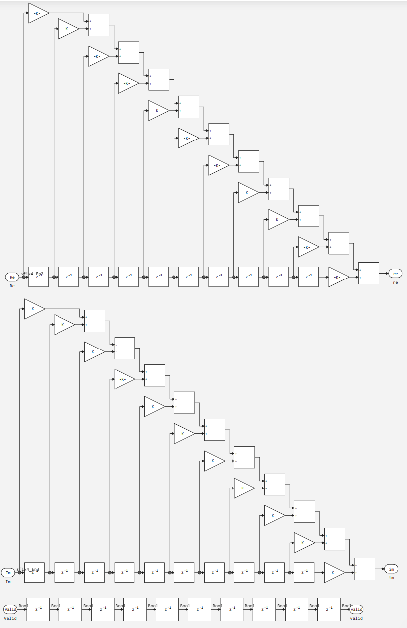
- FIR is a digital filter with finite impulse response that calculates each output value as a weighted sum of the last 11 input samples.
.png)
Now let's move on to launching the model and code generation.
function run_model( name_model)
    Path = (@__DIR__) * "/" * name_model * ".engee"
    if name_model in [m.name for m in engee.get_all_models()] # Checking the condition for loading a model into the kernel
        model = engee.open( name_model ) # Open the model
        model_output = engee.run( model, verbose=true ); # Launch the model
    else
        model = engee.load( Path, force=true ) # Upload a model
        model_output = engee.run( model, verbose=true ); # Launch the model
        engee.close( name_model, force=true ); # Close the model
    end
    sleep(0.1)
    return model_output
end
run_model("QPSK+FIR_verilog") # Launching the model.
Re = collect(simout["QPSK+FIR_verilog/FIR.re"]).value
Im = collect(simout["QPSK+FIR_verilog/FIR.im"]).value
plot(Re, label="Re")
plot!(Im, label="Im")
collect(simout["QPSK+FIR_verilog/FIR.re"]).value
The graphs will be useful for us to compare with the work of the Verilog code.
Now we will generate the code from the model blocks and describe the test module in the same way as the inputs to the model.
engee.generate_code(
"$(@__DIR__)/test_codgen_ic.engee",
"$(@__DIR__)/prj",
subsystem_name="QPSK_modulator"
)
engee.generate_code(
"$(@__DIR__)/test_codgen_ic.engee",
"$(@__DIR__)/prj",
subsystem_name="fir-1"
)
The tb module is a testbench that checks the operation of the QPSK modulator and FIR filter modules by feeding test data and recording the results.
The test bench supplies a cyclic sequence of bits to the input [11, 00, 10, 01], writes the output values of the modulator (QPSK_Re, QPSK_Im) and filter (FIR_Re, FIR_Im) to a file output_data.txt and it visualizes them in the console, and also generates the waveforms test file_codgen_ic.vcd for time chart analysis.
filename = "$(@__DIR__)/prj/tb.v"
try
    if !isfile(filename)
        println("The $filename file was not found!")
        return
    end
    println("The contents of the $filename file:")
    println("="^50)
    content = read(filename, String)
    println(content)
    println("="^50)
    println("End of file")
catch e
    println("Error reading the file: ", e)
end
Now let's run the simulation.
# Compilation
run(`iverilog -o sim tb.v QPSKFIR_verilog_FIR.v QPSKFIR_verilog_QPSK_modulator.v`)
# Running the simulation
run(`vvp sim`)
As we can see, based on the results of the simulation, 2 txt and vcd files were generated.
TXT is a text file with a data table (timestamps, signal values).
VCD (Value Change Dump) is a binary file of time diagrams used for visual debugging of signals in GTKWave and other analyzers.
Let's try to perform VCD parsing.
function vcd_to_txt(vcd_filename; output_txt="simple_output.txt")
    println("Simplified VCD to TXT conversion: ", vcd_filename)
    lines = readlines(vcd_filename)
    signals = Dict{String, Vector{Tuple{Float64, Any}}}()
    current_time = 0.0
    for line in lines
        line = strip(line)
        isempty(line) && continue
        if startswith(line, "\$var")
            parts = split(line)
            if length(parts) >= 4
                signal_id = parts[3]
                signal_name = parts[4]
                signals[signal_name] = []
            end
        elseif startswith(line, "#")
            current_time = parse(Float64, line[2:end])
        elseif length(line) >= 2
            value_char = line[1:1]
            signal_id = line[2:end]
            value = if value_char == "0"
                0
            elseif value_char == "1"
                1
            else
                0
            end
            for (name, values) in signals
                if occursin(signal_id, name) || signal_id == string(hash(name))[1:min(3, end)]
                    push!(values, (current_time, value))
                    break
                end
            end
        end
    end
    open(output_txt, "w") do io
        header = "Time\t" * join(keys(signals), "\t")
        println(io, header)
        all_times = Set{Float64}()
        for values in values(signals)
            for (time, _) in values
                push!(all_times, time)
            end
        end
        sorted_times = sort(collect(all_times))
        for time in sorted_times
            row = string(time)
            for signal_name in keys(signals)
                value = 0
                for (t, v) in signals[signal_name]
                    if t == time
                        value = v
                        break
                    elseif t < time
                        value = v
                    end
                end
                row *= "\t" * string(value)
            end
            println(io, row)
        end
    end
    println("Simplified conversion completed: ", output_txt)
end
vcd_to_txt("test_codgen_ic.vcd", output_txt="simple_result.txt")
As we can see, this is possible, but not very convenient and fast, plus we did not pull out the names of the fields.
So let's use the second option and analyze the TXT.
using DataFrames
using DelimitedFiles
using Plots

data = readdlm("output_data.txt", '\t', skipstart=1)  # Skipping the title
cycle = data[:, 1]
qpsk_re = data[:, 4]  # QPSK_Re in the 4th column
qpsk_im = data[:, 5]  # QPSK_Im in the 5th column
fir_re = data[:, 7]   # FIR_Re in the 7th column
fir_im = data[:, 8]   # FIR_Im in the 8th column

p = plot(layout=(2, 1), size=(800, 600))
plot!(p[1], cycle, qpsk_re, label="QPSK Real", linewidth=2, color=:blue)
plot!(p[1], cycle, qpsk_im, label="QPSK Imag", linewidth=2, color=:red)
title!(p[1], "QPSK Signal")
plot!(p[2], cycle, fir_re, label="FIR Real", linewidth=2, color=:green)
plot!(p[2], cycle, fir_im, label="FIR Imag", linewidth=2, color=:orange)
title!(p[2], "FIR Filter Output")
The verification results confirm that the behavior of the test case matches the expected model. Minor discrepancies are explained only by different types of data. The modules are working correctly: QPSK generates characters, and the FIR filter processes them.
Conclusion
In this example, we have analyzed how to visualize Verilog code simulation tests, and also generated a simple model of the transmission path of the communication system.