The workflow of system identification
Identification is the process of constructing a mathematical model of a dynamic object based on experimental data.
Pkg.add(["DataFrames", "CSV", "ControlSystemIdentification"])
using DataFrames, CSV, ControlSystemIdentification;
An approximate identification workflow looks like this: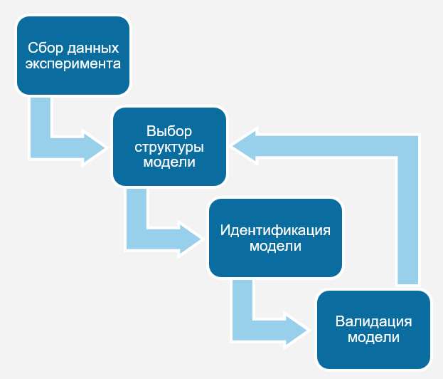
First, you need to conduct an experiment to collect system data. Then we select the structure of the model that we want to fit to this data and the identification algorithm. Next, the data obtained is "adjusted" to the selected structure. The identification result is checked against a validation dataset. If the identification result turns out to be unsatisfactory, it is necessary to go back and change the structure of the model or the identification algorithm.
Collecting experimental data
First of all, experimental data must be obtained for identification. In this example, the experiment data is uploaded to Engee from a CSV file. We will divide the experimental data into 2 parts: the first will be used for identification, the second for validation.
Import_data = "data.csv"
table = CSV.read(Import_data, DataFrame);
inputdata = Float64.(table[:, 2]);
outputdata = Float64.(table[:, 3]);
Identification data:
Ts = 0.1;
identdata  = iddata(outputdata[1:Int32(end/2)], inputdata[1:Int32(end/2)], Ts);
plot(identdata)
Validation data:
valdata  = iddata(outputdata[Int32(end/2):end], inputdata[Int32(end/2):end], Ts);
plot(valdata)
Model structure selection and identification
We will identify a linear stationary system in the state space. First, let's choose the order of the system equal to 1.
nx = 1; # system order
res = subspaceid(identdata, nx; verbose=true)
Validation of the model
simplot(valdata, res)
As we can see, the identified model does not sufficiently reproduce the dynamics of the real system.
Model structure modification and identification
Let's take a step back and change the structure of the model. Let the order of the system be 2 this time.
nx = 2; # system order
res = subspaceid(identdata, nx; verbose=true)
Validation of the model
simplot(valdata, res)
This time, we are satisfied with the accuracy of identification.
Conclusion
In this example, we got acquainted with the workflow of system identification based on experimental data obtained from the CSV table.