梯形(六步)BDPT控制(BLCD)
本项目展示了梯形(六步)控制模型[BDPT(BLDC)](https://engee.com/helpcenter/stable/cn/fmod-electricity-permanent-magnet/bldc.html )。
导言
梯形BDT控制是一个没有速度或电流反馈的系统.
确定电机轴位置的霍尔传感器仅用于切换电机绕组。 下图显示了这种管理模型的框图。
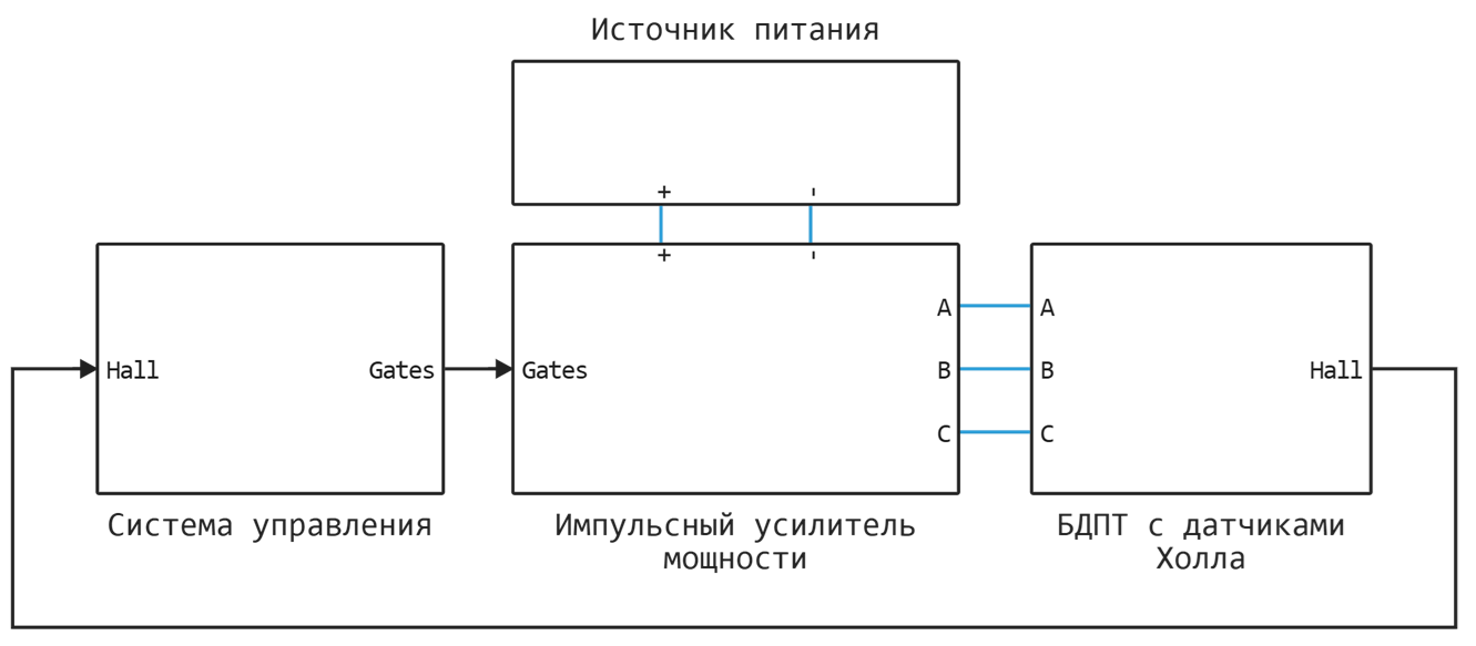
该模型由以下元素组成:
-控制系统(SU);
-开关功率放大器(IUM);
-电源(IP);
-带霍尔传感器的BDPT。
关键要素(CE)IUM是基于场效应晶体管(Mosfet)来选择的。
该模型实现了选择KE IUM的开关方法和控制方法以及BDPT相位的连接方案的可能性。
有关此处开发的模型所基于的电动机控制系统的更多信息,请参阅[1]。
管理系统
为这个例子开发的SU基于真值表(每个都有自己的控制方法),它们反过来定义了量化宽松和IUM的控制函数。
BDPT SU的装置如下所示。
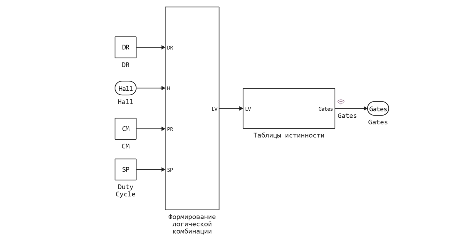
乂IUM的控制函数使用4个变量的逻辑组合形成:
DR-发动机的旋转方向(0-直接旋转,1-相反);H-霍尔传感器的位置信号;PR-定义KU IUM(PWM填充因子)的开关方法;SP-设置速度(PWM填充因子)。
KE和KUM切换方法
CE和IUM的切换方法影响CE之间的负载分配,并使用常数确定 CM. 采用三种切换方式:
-非对称(底部) CD = 0;
-不平衡(上) CD = 100;
-候补 CD = 50.
何时 CM = 0,这意味着 PR = 0,下层的负载比上层的负载更多。
在当 CM = 100, PR = 1 相反,较低的CES加载更多。
如果 CM = 50 并且,相应地, PR = 0,5,在PWM期间,上下两个CES相等地被加载。
管理CE和IUM的方法
控制面板有3种方式:120度,150度和180度。
控制方法由安装的霍尔传感器的数量及其相对位置决定。
在120度和180度控制方法中,需要将电机轴的位置分为6个扇区,为此需要安装3个霍尔传感器。
150度开关允许使用6个霍尔传感器,这意味着分成12个扇区。
例如,发动机模型中使用的传感器的位置如下所示,其中相位根据"星形"方案连接(wye)具有管理CE和IUM的各种方法。
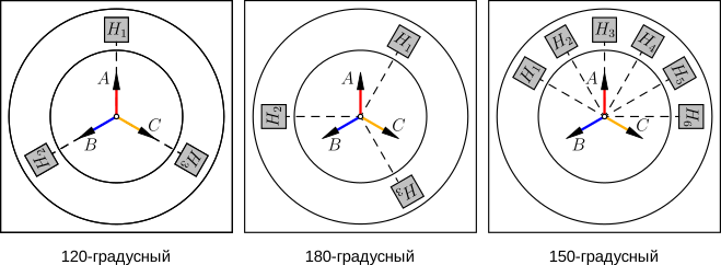
对于"三角形"连接图(Delta)所有霍尔传感器都旋转到 弧度顺时针方向。
使用霍尔传感器确定位置的算法基于它们相对于彼此的位移。
偏移如下所示 bias 霍尔传感器 H 当根据KE IUM的"star"方案和各种控制方法连接发动机的相位时。
H |
bias (120) |
bias (180) |
bias (150) |
|---|---|---|---|
H1 |
|||
H2 |
|||
H3 |
|||
H4 |
|||
H5 |
|||
H6 |
模拟仿真
我们将连接必要的扩展包:
# 添加丢失的软件包
Pkg.add(["CSV", "DataFrames"]);
# 连接必要的软件包
using CSV
using DataFrames
使用宏 @__DIR__ 定义项目文件路径的描述符:
demoroot = @__DIR__;
数据和参数
从真值表下载数据:
# 从CSV文件下载真值表
truthTable120d = CSV.read("$demoroot/data/truthTable120d.csv",
                         DataFrame; delim = ",", header = false);
truthTable150d = CSV.read("$demoroot/data/truthTable150d.csv",
                         DataFrame; delim = ",", header = false);
truthTable180d = CSV.read("$demoroot/data/truthTable180d.csv",
                         DataFrame; delim = ",", header = false);

# 管理QE IUM的方法
# #120度
tt120deg = truthTable120d.Column1;
tt120deg = [tt120deg truthTable120d.Column2];
tt120deg = [tt120deg truthTable120d.Column3];
tt120deg = [tt120deg truthTable120d.Column4];
tt120deg = [tt120deg truthTable120d.Column5];
tt120deg = [tt120deg truthTable120d.Column6];

# #150度
tt150deg = truthTable150d.Column1;
tt150deg = [tt150deg truthTable150d.Column2];
tt150deg = [tt150deg truthTable150d.Column3];
tt150deg = [tt150deg truthTable150d.Column4];
tt150deg = [tt150deg truthTable150d.Column5];
tt150deg = [tt150deg truthTable150d.Column6];

# #180度
tt180deg = truthTable180d.Column1;
tt180deg = [tt180deg truthTable180d.Column2];
tt180deg = [tt180deg truthTable180d.Column3];
tt180deg = [tt180deg truthTable180d.Column4];
tt180deg = [tt180deg truthTable180d.Column5];
tt180deg = [tt180deg truthTable180d.Column6];
我们将设置建模,IP,BDPT和IUM的参数:
# 仿真参数
Ts = 5e-6; # 物理模式的采样时间

# IP参数
Us = 24; # 电源电压,V

# BDPT参数
R  = 2.25;             # 定子绕组的电阻,欧姆
L  = 0.0032;           # 定子绕组的电感,Gn
Cm = 0.03397;          # 矩常数,N*m/A
Ce = 0.0258;           # 永久反EMF,V*s/rad
J  = 2.4e-6;           # 转子转动惯量,kg*m^2
Bm = 0;                # 转子阻尼,N*m*s/rad
p  = 4;                # 对极数
Fmax = (2/3)*(Cm/p);   # 永磁体磁通耦合的最大值
ThetaConst = pi/(2*p); # 电动势恒定的转子角度

# IUM参数
f     = 5000;  # 开关频率,Hz
Rds   = 4e-2;  # 漏源电阻,欧姆
Goffs = 1e-6;  # 关断状态下的电导率,Cm
Uthr  = 0.5;   # 阈值电压,V
Udf   = 0.8;   # 集成二极管的正向电压,在
Ron   = 1e-3;  # 直接接通时集成二极管的电阻,欧姆
Goff  = 1e-5;  # 集成二极管在闭合状态下的导电性,见
Csn   = 1e-7;  # 缓冲容量,F
Rsn   = 1e4;   # 缓冲电阻,欧姆
KE IUM的切换方法的选择是通过定义一个变量来进行的 comType 对应的编号(120/150/180).
# 选择CE和IUM的切换方式
comType = 120; # 120 / 150 / 180
同样,使用变量 woundType 发动机相的连接方案进行选择。 这里,"三角形"类型方案对应于 1,以及"明星"的类型 - 2.
# #电机相位连接方案的选择
woundType = 1; # 三角形=1,星形=2

# 如果AnyMath模型尚未在画布上打开,则加载该模型
if "bldc_control_sixstep" ∉ getfield.(engee.get_all_models(), :name)
    engee.load( "$demoroot/bldc_control_sixstep.engee");
end

bldc_root = "bldc_control_sixstep/БДПТ с датчиками Холла/БДПТ";
if woundType == 1
    engee.set_param!(bldc_root, "winding_type" => "Delta-wound")
elseif woundType == 2
    engee.set_param!(bldc_root, "winding_type" => "Wye-wound")
    engee.set_param!(bldc_root, "zero_sequence" => "Exclude")
end
最后,我们定义切换方法CE和IUM的变量 CM,方向 DR 和速度 SP 电机轴的旋转:
CM = 0;   # 0-不平衡(下)100-不平衡(上),50-交替
DR = 0;   # 0-正向旋转,1-反向
SP = 100; # PWM[0...100]-发动机最大转速的%
打开模型并运行仿真。:
# 运行AnyMath模型的模拟
model_data = engee.run("bldc_control_sixstep");
让我们提取模拟过程中获得的数据。:
angle = model_data["Angle"].value;  # 电机轴的旋转角度,deg
speed = model_data["Speed"].value;  # 发动机轴转速,rpm

# 电流
is = model_data["is"].value;  # 从IP消耗电流
ia = model_data["ia"].value;  # A相电流
ib = model_data["ib"].value;  # B相电流
ic = model_data["ic"].value;  # C相电流

# 电压;电压
Ua = model_data["Ua"].value;   # 相电压A
Ub = model_data["Ub"].value;   # 相电压B
Uc = model_data["Uc"].value;   # 相电压C
Uab = model_data["Uab"].value; # 线电压C
Ubc = model_data["Ubc"].value; # 线电压C
Uca = model_data["Uca"].value; # 线电压C

# 霍尔传感器H
Hall = model_data["Hall"].value;

Hall_1 = zeros(Float64, length(Hall));
Hall_2 = zeros(Float64, length(Hall));
Hall_3 = zeros(Float64, length(Hall));

for i = 1:length(Hall)
    Hall_1[i] = Hall[i][1];
    Hall_2[i] = Hall[i][2];
    Hall_3[i] = Hall[i][3];
end

if comType == 150
    Hall_4 = zeros(Float64, length(Hall));
    Hall_5 = zeros(Float64, length(Hall));
    Hall_6 = zeros(Float64, length(Hall));

    for i = 1:length(Hall)
        Hall_4[i] = Hall[i][4];
        Hall_5[i] = Hall[i][5];
        Hall_6[i] = Hall[i][6];
    end
end

# G的关键要素
Gates = model_data["Gates"].value;

Gates_1 = zeros(Float64, length(Gates));
Gates_2 = zeros(Float64, length(Gates));
Gates_3 = zeros(Float64, length(Gates));
Gates_4 = zeros(Float64, length(Gates));
Gates_5 = zeros(Float64, length(Gates));
Gates_6 = zeros(Float64, length(Gates));

for i = 1:length(Gates)
    Gates_1[i] = Gates[i][1];
    Gates_2[i] = Gates[i][2];
    Gates_3[i] = Gates[i][3];
    Gates_4[i] = Gates[i][4];
    Gates_5[i] = Gates[i][5];
    Gates_6[i] = Gates[i][6];
end
结果
让我们绘制BDPT转子的位置和速度。:
# gr()#绘制图形时禁用交互性(更容易绘制)
plotlyjs() # 启用交互性(更难绘制)
t = model_data["Angle"].time; # 模拟时间,s
plot(
    plot(t, angle, ylabel = "旋转角度,度", lw = 1.5, c = "red",
    title = ""),
    plot(t, speed, xlabel = "时间,从", lw = 1.5, c = "green",
    ylabel = "Скорость, об/мин"),
    layout = (2,1), legend=:false, link=:x
)
相电流和电源电流图:
# gr()#绘制图形时禁用交互性(更容易绘制)
plotlyjs() # 启用交互性(更难绘制)
t = model_data["is"].time; # 模拟时间,s
plot(
    plot(t, is, ylabel = "电源,以及", lw = 1.5, c = "black",
    title = "电流"),
    plot(t, [ia, ib, ic], lw = 1.5, c = ["red" "blue" "yellow"],
    xlabel = "时间,从", ylabel = "以相位为基础,以及"),
    layout = (2,1), legend=:topright, label = ["is" "ia" "ib" "ic"], link=:x
)
以下是电机电压、霍尔传感器信号和控制面板上的图表。
# gr()#绘制图形时禁用交互性(更容易绘制)
plotlyjs() # 启用交互性(更难绘制)
t = model_data["Ua"].time; # 模拟时间,s
plot(
    plot(t, [Ua, Ub, Uc], ylabel = "阶段,在", lw = 1.5, c = ["red" "blue" "yellow"],
    title = "BDPT电压", label = ["Ua" "Ub" "Uc"]),
    plot(t, [Uab, Ubc, Uca], lw = 1.5, c = ["red" "blue" "yellow"],
    xlabel = "时间,从", ylabel = "线性的,在", label = ["Uab" "Ubc" "Uca"]),
    layout = (2,1), legend=:right, link=:x
)
# gr()#绘制图形时禁用交互性(更容易绘制)
plotlyjs() # 启用交互性(更难绘制)
t = model_data["Hall"].time; # 模拟时间,s
if comType == 150
plot(
    plot(t, Hall_1, ylabel = "H1", lw = 1.5,
    title = "来自霍尔传感器的信号"),
    plot(t, Hall_2, lw = 1.5,
    ylabel = "H2"),
    plot(t, Hall_3, lw = 1.5,
    ylabel = "H3"),
    plot(t, Hall_4, lw = 1.5,
    ylabel = "H4"),
    plot(t, Hall_5, lw = 1.5,
    ylabel = "H5"),
    plot(t, Hall_6, lw = 1.5,
    ylabel = "H6", xlabel = "时间,从"),
    layout = (6,1), legend=:none, link=:x
)
else
    plot(
        plot(t, Hall_1, ylabel = "H1", lw = 1.5,
        title = "来自霍尔传感器的信号"),
        plot(t, Hall_2, lw = 1.5,
        ylabel = "H2"),
        plot(t, Hall_3, lw = 1.5,
        ylabel = "H3", xlabel = "时间,从"),
        layout = (3,1), legend=:none, link=:x
    )
end
# gr()#绘制图形时禁用交互性(更容易绘制)
plotlyjs() # 启用交互性(更难绘制)
t = model_data["Gates"].time; # 模拟时间,s
plot(
    plot(t, Gates_1, ylabel = "G1", lw = 1.5,
    title = "KE IUM上的信号"),
    plot(t, Gates_2, lw = 1.5,
    ylabel = "G2"),
    plot(t, Gates_3, lw = 1.5,
    ylabel = "G3"),
    plot(t, Gates_4, lw = 1.5,
    ylabel = "G4"),
    plot(t, Gates_5, lw = 1.5,
    ylabel = "G5"),
    plot(t, Gates_6, lw = 1.5,
    ylabel = "G6", xlabel = "时间,从"),
    layout = (6,1), legend=:none, link=:x
)
结论
该项目展示了一个6步BDT开关模型(BLDC)。
考虑了这种类型的控制的结构,操作原理和执行选项。
仿真结果得到了来自霍尔传感器和直流转换器关键元件的电流、电压和逻辑信号图。
所开发的模型例如可用作电驱动器的致动元件。
使用的来源列表
- *Krivilev A.V.*基于计算机辅助的"功率放大器—电动机"系统脉冲控制节能方法的Fpga开发与实现
设计方法:技术科学博士论文摘要。科学,莫斯科:MAI,2013。