Simulation of the PDSCH 5G NR transmission path

Physical Downlink Shared Channel (PDSCH) is the main data transmission channel in the 5G downlink NR. Its performance is critical for network bandwidth and latency. The design of PDSCH is difficult due to the need for coordinated work of the encoding, modulation, spatial processing (MIMO) and resource allocation processes of OFDM.

The article presents a PDSCH transmitter model that implements a complete signal processing path in accordance with **the basic principles of ** 3GPP. The model includes transport block generation, channel coding (DL-SCH), QPSK modulation, spatial precoding for the MIMO 8x5 configuration, resource grid generation, and OFDM modulation. The model configuration uses realistic parameters: 51 resource blocks and a subcarrier pitch of 30 kHz.

using LinearAlgebra, Statistics, Dates, EngeeDSP

# Enabling the auxiliary model launch function.
function run_model( name_model)
    Path = (@__DIR__) * "/" * name_model * ".engee"
    if name_model in [m.name for m in engee.get_all_models()] # Checking the condition for loading a model into the kernel
        model = engee.open( name_model ) # Open the model
        model_output = engee.run( model, verbose=true ); # Launch the model
    else
        model = engee.load( Path, force=true ) # Upload a model
        model_output = engee.run( model, verbose=true ); # Launch the model
        engee.close( name_model, force=true ); # Close the model
    end
    sleep(0.1)
    return model_output
end

run_model (generic function with 1 method)

Description of the model and functional blocks

The model is an end-to-end simulation chain of the PDSCH 5G NR transmitter, which implements signal processing from data bits to a multi-channel OFDM signal. The architecture is modular, each block corresponds to a processing stage according to 3GPP specifications. The model implements the 5G NR standard in detail, serving as a tool for analyzing, training, and verifying physical layer algorithms.

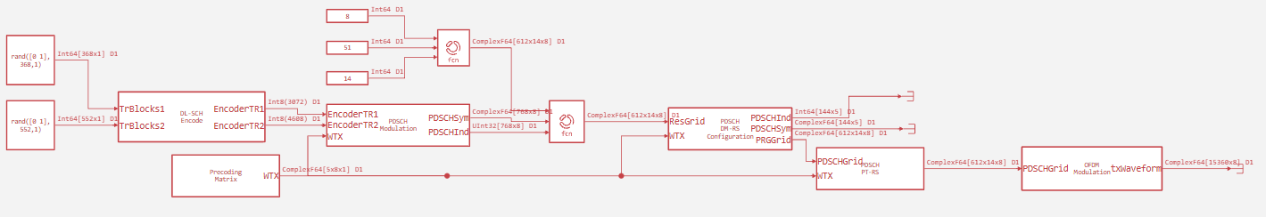
Data generation and processing

TrBlocks, TrBlocks-1: Generate test transport blocks (368 and 552 bits).
DL-SCH Encode: Performs channel encoding: CRC addition, LDPC encoding, scrambling.

Signal generation and spatial processing

PDSCH Modulation: Performs QPSK modulation by converting bits into complex symbols.
Precoding Matrix: Calculates the precoding matrix for the MIMO 5x8 configuration, providing spatial multiplexing.

Working with the resource grid

Create resource grid: Creates an empty three-dimensional resource grid (612×14×8) for one slot.
PDSCH mapping in grid: Places modulated PDSCH symbols in designated grid cells.

Formation of reference signals

PDSCH DM-RS Configuration: Generates and places demodulation reference signals (DM-RS) based on precoding.
PDSCH PT-RS-1: Block for phase noise compensation reference signals (disabled in the model).

Final signal generation

OFDM Modulation: Performs IFFT and adds a cyclic prefix, forming a multi-channel time signal for transmission.
Configuration blocks (Constant): The main parameters are set: carrier size, number of characters, number of antennas.

The model is run and the results are extracted for further analysis.

simout = run_model("NR_PDSCH_Throughput") — start the simulation.
Extraction of key output signals:
- precoding_matrix — the MIMO precoding matrix.
- encoded_tr1, encoded_tr2 — encoded transport blocks.
- ofdm_waveform — multi-channel OFDM signal.
- pdsch_grid, dmrs_grid, final_grid — resource grids at different stages.

simout = run_model("NR_PDSCH_Throughput")

precoding_matrix = collect(simout["Precoding Matrix.WTX"]).value[end]
encoded_tr1 = collect(simout["DL-SCH Encode.EncoderTR1"]).value[end] 
encoded_tr2 = collect(simout["DL-SCH Encode.EncoderTR2"]).value[end]  
ofdm_waveform = collect(simout["OFDM Modulation.txWaveform"]).value[end]
pdsch_grid = collect(simout["PDSCH mapping in grid associated with PDSCH transmission period.1"]).value[end]
dmrs_grid = collect(simout["PDSCH DM-RS Configuration.PRGGrid"]).value[end]
final_grid = collect(simout["PDSCH PT-RS-1.1"]).value[end];

Building...
Progress 0%
Progress 100%

The presented code performs a comprehensive analysis of the model's output data. Source of configuration parameters num_layers=5, num_antennas=8, n_size_grid=51, scs=30 taken directly from the settings of the model blocks (for example, "DL-SCH Encode", "Precoding Matrix").

A brief description of the analysis being performed:

System configuration: Output of the main parameters of the model.
Signal dimensions: Checking the correctness of output data formats.
Performance metrics:

Calculation of the total amount of transferred data.
- Assessment of the efficiency of using the resource grid (the ratio of occupied elements to the total number).

MIMO precoding analysis:
- Calculation of precoding matrix norms for each layer.
- Estimation of the deviation of the matrix from orthogonality/unitarity.
Characteristics of the OFDM signal:

Calculation of the peak factor coefficient (PAPR) and average power for each antenna.

Comparison of resource grids: Determination of the share of service signals (DM-RS) in the final grid.

num_layers = 5      # Number of spatial MIMO layers
num_antennas = 8    # Number of transmitting antennas
n_size_grid = 51    # Carrier size in resource blocks (RB)
scs = 30            # Subcarrier pitch (kHz)

println("\n1. SYSTEM CONFIGURATION:")
println("   • MIMO: $num_layers of layers × $num_antennas of antennas")
println("   • Carrier: $n_size_grid RB, subcarrier pitch $scs kHz")
println("   • Modulation: QPSK")
println("   • Transport blocks: $(length(encoded_tr1)) and $(length(encoded_tr2)) bits")

println("2. SIGNAL DIMENSIONS:")
println("   • Precoding matrix: $(size(precoding_matrix)) (layers×antennas×subcarriers)")
println("   • OFDM signal: $(size(ofdm_waveform)) (counts×antennas)")
println("   • PDSCH resource grid: $(size(pdsch_grid)) (subcarriers×OFDM symbols×antennas)")
println("   • Final resource grid: $(size(final_grid)) (subcarriers×OFDM symbols×antennas)")

println("3. PERFORMANCE METRICS:")
println("   " * "-"^45)

total_bits = length(encoded_tr1) + length(encoded_tr2)
println("   • Total amount of data: $total_bits bits ($(round(total_bits/8, digits=2)) bytes)")

K, L, P = size(final_grid)
total_resource_elements = K * L * P
occupied_elements = count(!iszero, final_grid)
resource_utilization = occupied_elements / total_resource_elements * 100

println("   • Total resource elements: $total_resource_elements")
println("   • Resource elements are occupied: $occupied_elements")
println("   • Resource efficiency: $(round(resource_utilization, digits=2))%")

println("4. MIMO PRECODING ANALYSIS:")
precoding_norms = [norm(precoding_matrix[layer, :, :]) for layer in 1:num_layers]
println("   • Precoding standards by layers:")
for (i, norm_val) in enumerate(precoding_norms)
    println("     Layer $i: $(round(norm_val, digits=4))")
end

if size(precoding_matrix, 1) <= size(precoding_matrix, 2)
    W = precoding_matrix[:, :, 1]
    if size(W, 1) < size(W, 2)
        deviation = norm(W' * W - Diagonal(diag(W' * W)))
        println("   • Deviation from column orthogonality: $(round(deviation, digits=6))")
    else
        deviation = norm(W' * W - I)
        println("   • Deviation from unitarity: $(round(deviation, digits=6))")
    end
end

println("5. CHARACTERISTICS OF THE OFDM SIGNAL:")
peak_to_average_ratios = Float64[]
average_powers = Float64[]

for ant in 1:num_antennas
    signal = ofdm_waveform[:, ant]
    papr = 10 * log10(maximum(abs2.(signal)) / mean(abs2.(signal)))
    avg_power = 10 * log10(mean(abs2.(signal)))
    push!(peak_to_average_ratios, papr)
    push!(average_powers, avg_power)
end

println("   • Average PAPR for antennas: $(round(mean(peak_to_average_ratios), digits=2)) dB")
println("   • Average antenna power: $(round(mean(average_powers), digits=2)) dB")
println("   • Power range: $(round(minimum(average_powers), digits=2)) - $(round(maximum(average_powers), digits=2)) dB")

println("6. COMPARISON OF RESOURCE GRIDS:")
if size(pdsch_grid) == size(final_grid)
    data_only_elements = count(!iszero, pdsch_grid)
    final_elements = count(!iszero, final_grid)
    added_elements = final_elements - data_only_elements
    
    println("   • Items with PDSCH data only: $data_only_elements")
    println("   • Total items in the final grid: $final_elements")
end

1. КОНФИГУРАЦИЯ СИСТЕМЫ:
   • MIMO: 5 слоев × 8 антенн
   • Несущая: 51 RB, шаг поднесущей 30 кГц
   • Модуляция: QPSK
   • Транспортные блоки: 3072 и 4608 бит

2. РАЗМЕРНОСТИ СИГНАЛОВ:
   • Матрица прекодирования: (5, 8, 1) (слои×антенны×поднесущие)
   • OFDM сигнал: (15360, 8) (отсчеты×антенны)
   • Ресурсная сетка PDSCH: (612, 14, 8) (поднесущие×OFDM-символы×антенны)
   • Финальная ресурсная сетка: (612, 14, 8) (поднесущие×OFDM-символы×антенны)

3. МЕТРИКИ ПРОИЗВОДИТЕЛЬНОСТИ:
   ---------------------------------------------
   • Общий объем данных: 7680 бит (960.0 байт)
   • Всего ресурсных элементов: 68544
   • Занято ресурсных элементов: 8448
   • Эффективность использования ресурсов: 12.32%

4. АНАЛИЗ ПРЕКОДИРОВАНИЯ MIMO:
   • Нормы прекодирования по слоям:
     Слой 1: 0.4472
     Слой 2: 0.4472
     Слой 3: 0.4472
     Слой 4: 0.4472
     Слой 5: 0.4472
   • Отклонение от ортогональности столбцов: 0.269838

5. ХАРАКТЕРИСТИКИ OFDM СИГНАЛА:
   • Средний PAPR по антеннам: 10.96 dB
   • Средняя мощность по антеннам: -51.19 dB
   • Диапазон мощностей: -52.05 - -50.51 dB

6. СРАВНЕНИЕ РЕСУРСНЫХ СЕТОК:
   • Элементы только с данными PDSCH: 8448
   • Всего элементов в финальной сетке: 8448

The analysis confirms the correct operation of the basic model of the PDSCH transmitter. The model successfully processes two transport blocks with a total volume of 7680 bits. The efficiency of using the resource grid was 12.32%, which corresponds to the specifics of the test scenario with partial filling of resource blocks.

The precoding matrix demonstrates a uniform distribution of power over five spatial layers with a moderate deviation from orthogonality (0.27), which is acceptable for the basic MIMO scheme.

The characteristics of the OFDM signal correspond to expectations: the peak factor of ~11.1 dB is typical for OFDM systems, the signal power is evenly distributed over the antennas. The current model configuration forms a resource grid containing only PDSCH data.

The model successfully implements the main transmission path and serves as the basis for extending functionality, including adding overhead signals and analyzing complex scenarios.

The code below creates a graph showing how the amount of information changes at different stages of processing in the PDSCH transmitter. The logarithmic scale shows the increase in the number of elements from the initial bits (920) to the final samples of the OFDM signal (122,880). The graph clearly demonstrates the increase in data at the stages of encoding and modulation, as well as the conversion of discrete characters into an analog time signal.

stages = ["Input TBs", "Encoded TBs", "Modulated symbols", "Resource Grid", "OFDM signal"]
tb1_bits = 368
tb2_bits = 552
total_input_bits = tb1_bits + tb2_bits
encoded_bits = length(encoded_tr1) + length(encoded_tr2)
modulated_symbols = encoded_bits ÷ 2
grid_symbols = occupied_elements
ofdm_samples = size(ofdm_waveform, 1) * size(ofdm_waveform, 2)
sizes = [total_input_bits, encoded_bits, modulated_symbols, grid_symbols, ofdm_samples]

plot1 = plot(stages, sizes, seriestype=:scatter, markersize=8, linewidth=2, marker=:circle,
             title="The evolution of data volume", xlabel="Processing stage", ylabel="Number of elements",
             legend=false, yscale=:log10, grid=true)
plot!(stages, sizes, linewidth=1.5, color=:blue, alpha=0.5)

for i in 1:length(stages)
    annotate!(plot1, i, sizes[i]*1.1, text("$sizes[i]", 8, :bottom))
end

display(plot1)

The code below creates a heat map for visualizing the phase angles of the precoding matrix, where the Y—axis corresponds to the MIMO layers (1-5) and the X-axis to the transmitting antennas (1-8).

W = precoding_matrix[:, :, 1]
plot2 = heatmap(angle.(W), 
                title="The phase of the pre-coding matrix", 
                xlabel="Antennas", ylabel="Layers", 
                color=:hsv, clim=(-π, π),
                size=(600, 400),
                aspect_ratio=:auto)

display(plot2)

The analysis of the phase pattern shows a typical structure for the basic precoding matrix in the MIMO 5x8 system. The phase range covers almost a full circle from -177.8° to 180°, which is expected since the elements of the matrix are complex numbers with arbitrary phases. However, the average phase value of 13.6° indicates a slight shift in the distribution. A critical observation is that for each layer, the first antenna (column 1) has a fixed phase of 0° (or 180° for layer 4), which is a standard normalization technique that serves as a phase reference for the entire system.

Further, the antenna phases for each layer vary in a wide range, forming unique patterns: for example, in layer 2 there is a sharp transition from negative phases to positive (~ 100 °), and in layer 3 there are almost opposite phases (-177.8 ° and 176.8 °).

Such a variety of phase profiles between the layers confirms that the matrix implements spatial multiplexing, directing each data stream (layer) with a different phase weighting to the antenna array. The absence of an obvious linear phase progression across the antennas (which is typical for simple beamforming) is consistent with the goal of simultaneous transmission of several independent streams. Thus, visualization confirms that the precoding matrix correctly forms five spatially spaced channels.

The code below plots the signal power distribution across 8 transmitting antennas after the MIMO precoding operation. The uniform height of the columns on the graph confirms the balanced use of the antenna array, which is a prerequisite for efficient spatial multiplexing.

antenna_power = [norm(W[:,j]) for j in 1:size(W,2)]
plot3 = bar(antenna_power, 
            title="Antenna power", 
            xlabel="The antenna", ylabel="Power", 
            color=:red, alpha=0.7, 
            legend=false,
            size=(600, 400))

display(plot3)

The code below performs spectral analysis of the OFDM signal for the first two antennas. Using a spectrum analyzer, he plots the dependence of power (in dBm) on the frequency in the band. The spectra show the shape and bandwidth of the generated signal.

fs_hz = 30.72e6
n_antennas = size(ofdm_waveform, 2)
antennas_to_plot = 2

plot4 = plot(title="OFDM signal Spectrum", 
             xlabel="Frequency (MHz)", 
             ylabel="Power (dBm)", 
             grid=true, 
             legend=true,
             size=(800, 500))

colors = [:blue, :red, :green, :orange, :purple, :brown, :pink, :gray]

for ant in 1:min(antennas_to_plot, n_antennas)
    iq_data = ofdm_waveform[:, ant]
    RBW = fs_hz / 4096
    
    scope = EngeeDSP.spectrumAnalyzer()
    scope.SampleRate = fs_hz
    scope.Method = "filter-bank"
    scope.FrequencySpan = "full"
    scope.RBWSource = "property"
    scope.RBW = RBW
    scope.SpectrumType = "power"
    scope.SpectrumUnits = "dBm"
    scope.Window = "Kaiser"
    scope(iq_data)
    
    spectrumdata = EngeeDSP.getSpectrumData(scope)
    frequencies_mhz = spectrumdata["frequencies"] / 1e6
    
    plot!(plot4, frequencies_mhz, spectrumdata["spectrum"], 
          linewidth=1.5, label="Antenna $ant", color=colors[mod1(ant, length(colors))])
end

display(plot4)

Conclusion

The paper develops, implements and analyzes a model of the transmission path of the PDSCH channel of the 5G NR standard. The model correctly reproduces the full signal processing cycle in accordance with 3GPP specifications for a realistic MIMO 8x5 configuration with 51 RB carrier and 30 kHz subcarrier pitch.

The simulation results confirm the operability of all key stages: from LDPC channel coding and QPSK modulation to spatial precoding and OFDM modulation. All signal metrics (peak factor, power and phase distribution, resource efficiency) are within the expected limits and comply with the principles of operation of the physical layer.