Designing a smartphone camera focusing system
We will connect the necessary libraries.
import Pkg;
Pkg.add(["ControlSystemIdentification", "ControlSystems"])
using ControlSystems                # the main library for working with ACS
using ControlSystemIdentification   # a library for evaluating dynamic models based on data
Management object
The model shown below simulates the autofocus control system of a smartphone camera.
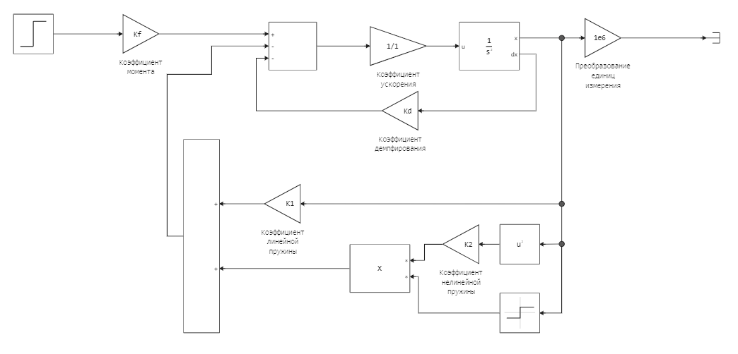
Consider the smartphone's autofocus model. The smartphone's electronics control the motor through feedback from the camera. Let's abstract from the technology and say that we need the transition process to take no more than 0.6 seconds from the moment we receive the focus command. Using the PID controller, we will try to implement such a system.
Our motor-lens system is non-linear, so first of all we linearize the model.
Linearization of the control object
Let's run the model using team management. As a result, we get a variable in the workspace data, which contains the simulation results.
modelName = "lens"
if !(modelName in [m.name for m in engee.get_all_models()]) engee.load( "$(@__DIR__)/$(modelName).engee"); end;
data = engee.run( modelName )
Let's write the data of the input and output signals into variables and plot them on a graph.
dataIn = collect(data["Step function.1"]).value;
dataOut = collect(data["Conversion of units of measurement.1"]).value;
data_t = collect(data["Conversion of units of measurement.1"]).time;

plot( data_t, [dataIn dataOut], label=["The input signal" "The output signal"] )
Let's move on to the linearization of the model. All methods for identifying the library model ControlSystemIdentification they accept an AbstractIdData type object as input. The function allows you to get an object of time domain identification data iddata. Next, using the method subspaceid we obtain a description of the system in the form of a state space.
Ts = data_t[2] - data_t[1]                     # We obtain the sampling frequency of the system from the time vector
d  = iddata(dataOut, dataIn, Ts);              # creating a data identification object in the time space
sys_d = subspaceid(d, :auto);                  # launching the state space model identification method
Let's compare the resulting model description with the model assembled in the modeling environment. To do this, use the block Пространство состояний and as the values of the matrices, we will write down the obtained values A,B,C,D.
sys = d2c(sys_d);   # let's move on to the continuous model
A = sys.A;          # we find the matrix A
B = sys.B;          # we find the matrix B
C = sys.C;          # we find the matrix C
D = sys.D;          # we find the matrix D
Selection of coefficients: the pid() function
To assess how suitable the selected coefficient values are, we will plot the LFX, LFX and Nyquist hodograph. And also to evaluate the quality of the transition process. For convenient display of frequency response graphs, the function is implemented below pid_marginplot. It substitutes the values of the resulting board system into a function for constructing frequency characteristics.: marginplot and nyquistplot, and displays them on graphs.
function pid_marginplot(C)
    f1 = marginplot(sys_tf * C, w)
    f2 = nyquistplot(sys_tf * C, xlims=(-10,1), ylims=(-2, 10), title="")
    plot(f1,f2, titlefontsize=10)
end
Setting additional variables. Let's transform the representation of the system into a transfer function and set the frequencies for which we will build time and frequency characteristics.
sys_tf = tf(sys);
w = exp10.(LinRange(-2.5, 3, 500));
We will set the coefficients using the cell mask. By moving the sliders, you set a new variable value. When one coefficient is changed, the code under the mask is recalculated. If you want to change several parameters at once, disable auto-refresh under the cell start button and start the cell manually.
The selection of coefficients is iterative, so first we will evaluate the characteristics of the system without a regulator, then we will begin to change each one and evaluate the impact of changes on the system.
kp = 0.4 # @param {type:"slider", min:0.1, max:5, step:0.1}
ki = 1.322 # @param {type:"slider", min:0.0, max:20, step:0.001}
kd = 0.03 # @param {type:"slider", min:0.0, max:0.5, step:0.01}
Tf = 0.012 # @param {type:"slider", min:0.0, max:1, step:0.001}

C0 = pid(kp, ki, kd; Tf, form=:parallel, filter_order=2)
pid_marginplot(C0)
Let's check if our system is stable. This allows you to do the function isstable.
isstable(feedback(sys_tf * C0)) # Verification: is the system stable with the received PID controller
Further, if the system is stable and the stability reserves meet our requirements, we will build a transition process and evaluate the quality of its characteristics.
plot(stepinfo(step(feedback(sys_tf * C0), 5))) # Assessment of the ACS transition process
The obtained controller data can be used for a model in a simulation environment. To do this, you can take the coefficient values from the workspace and specify them in the PID controller block.
Coefficient selection: loopshapingPID() function
Selection of coefficients using the function loopshapingPID It is based on the frequency approach (Loop Shaping), which allows you to set the desired frequency response of an open-loop system to ensure the desired characteristics of a closed loop. Thus, this method is convenient if the desired frequency properties of the system are known (for example, the required bandwidth or the level of disturbance suppression).
Let's try to apply this method to our example and get the desired characteristics.
The function takes a description of the system in the form of a transfer function and the frequency at which it is desirable to achieve a single gain of the open system. Additionally, the function accepts the parameter values of the additional sensitivity function Mt and the desired phase shift ϕt. By default, these parameters have optimal values, but they can be changed. You can also adjust the shape of the synthesized PID controller and display graphs that will help evaluate the quality of the resulting ACS.
ω  = 17
Tf = 1/1000ω
C0, kp, ki, kd, fig, CF = loopshapingPID(sys_tf, ω; Mt = 1.3, ϕt = 75, form=:parallel, doplot = true)
Let's try to change the frequency. If we analyze the Nyquist diagram, we can see that the characteristic passes very close to the critical point. Let's try to adjust this and install ω = 17. Now the characteristic of the adjusted system will touch the circle Mt at the point where ω = 17 at an angle ϕt = 75.
plot(fig)
Let's make sure that the resulting system is stable.
isstable(feedback(CF*sys_tf))
We will build LCH and LFCH systems and reflect the reserves of sustainability.
marginplot([sys_tf, CF*sys_tf])
We will also postulate the transition process of the received ACS. We see that the transition time is about 0.4 seconds, which meets our requirements.
plot(stepinfo(step(feedback(CF * sys_tf), 1)))
Using the obtained PID controller, we will simulate the system in a simulation environment. And we will display the results on a graph.
tuned_mdl = engee.load(joinpath("$(@__DIR__)","lens_pid.engee");force=true)
res = engee.run(tuned_mdl);
res_step = collect(res["Step function.1"]);
res_out = collect(res["Conversion of units of measurement.1"]);
plot(res_step.time, [res_step.value res_out.value], label=["The input signal" "The output signal"])