数字信号处理(DSP)入门 AnyMath

使用函数

信号加载和可视化

功能 使用 使列出的模块可供用户使用，类似于功能 进口 在其他语言:

不必像在MATLAB中那样将多个输出括在括号中。

using DSP, WAV
plotly()

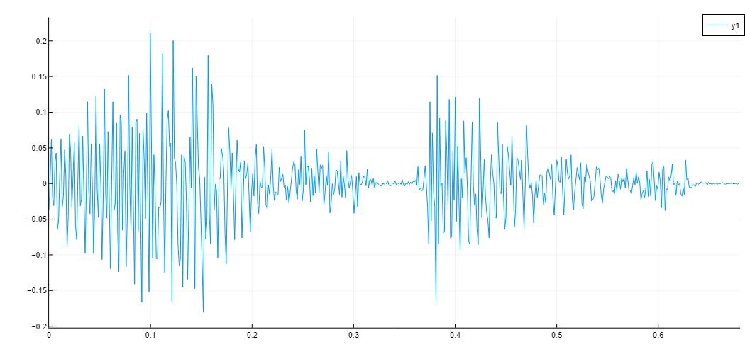
s, fs = wavread("/user/test.wav")

plot(0:1/fs:(size(s,1)-1)/fs, s)

输出

getting started dsp 1

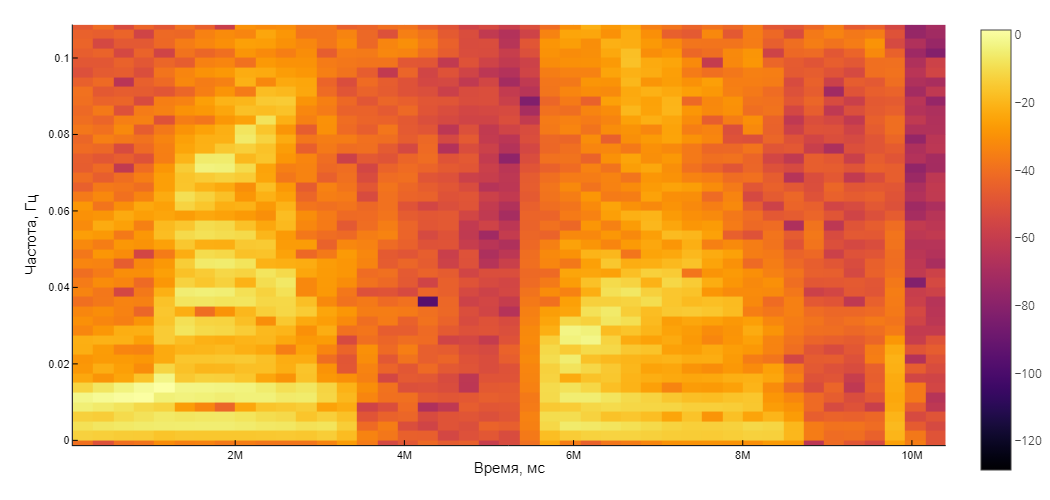
下面的函数接受一个带有语音标准参数的频谱图（汉宁窗） 25毫秒，重叠 10毫秒），构建并返回一个频谱图:

S = spectrogram(s[:,1], convert(Int, 25e-3*fs), convert(Int, 10e-3*fs); window=hanning)
Plots.heatmap(S.time.*1000, S.freq, pow2db.(S.power), xguide = "Время, мс", yguide = "Частота, Гц")

输出

getting started dsp 2

信号处理

现在让我们将信号通过滤波器来模拟手机的带宽，并再次构建其频谱图。:

responsetype = Bandpass(300, 3400; fs=fs)
prototype = Butterworth(8)
telephone_filter = digitalfilter(responsetype, prototype)

让我们来看看过滤器的特性:

变量可以具有Unicode名称。这被键入为\omega+tab。

ω = 0:0.01:pi
H = freqz(telephone_filter, ω)

过滤我们的信号:

sf = filt(telephone_filter, s)

Sf = spectrogram(s[:,1], convert(Int, 25e-3*fs), convert(Int, 10e-3*fs); window=hanning)
Plots.heatmap(Sf.time.*1000, Sf.freq, pow2db.(Sf.power), xguide = "Время, мс", yguide = "Частота, Гц")

输出

getting started dsp 3

再现结果

using Base64

function audioplayer(filepath)
  markup = """<audio controls="controls" {autoplay}>
        <source src="$filepath" />
        Your browser does not support the audio element.
        </audio>"""

  display(MIME("text/html") ,markup)
 end

 function audioplayer(s, fs)
  buf = IOBuffer()
  wavwrite(s, buf; Fs=fs)
  data = base64encode(unsafe_string(pointer(buf.data), buf.size))
  markup = """<audio controls="controls" {autoplay}>
        <source src="data:audio/wav;base64,$data" type="audio/wav" />
        Your browser does not support the audio element.
        </audio>"""
  display(MIME("text/html") ,markup)
end

audioplayer(s, fs)
audioplayer(sf, fs)

输出

音频::图像$getting-started-dsp/example-file.波[] 音频::image$getting-started-dsp/example-file-1。波[]

信号过采样

在这个例子中，我们将考虑从一个频率重新采样音频信号。 48千赫 在频率上 44.1千赫 采用低通滤波器的开发，随后进行信号过采样。

让我们找到插值和抽取的系数。

using Plots
using DSP

Fdat = 48e3;
Fcd = 44.1e3;
LM = Rational{Int32}(Fcd/Fdat);
L = LM.num;
M = LM.den;
(L,M)

输出

(147, 160)

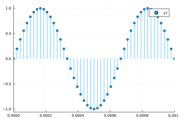
可视化原始音频信号:

t = 0:1/Fdat:0.25-1/Fdat;
x = sin.(2*pi*1.5e3*t);
gr()
plot(t, x, line=:stem, marker=:circle)
xlims!((0,0.001))

输出

getting started dsp 4

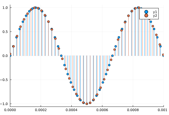
我们将做过采样并将接收到的信号叠加在原始信号上。

f = (Fdat/2)*min(1/L,1/M)
win = DSP.Windows.kaiser(3579,3);
fir = DSP.Filters.digitalfilter(DSP.Filters.Lowpass(f/48e3),FIRWindow(win)).

xup = DSP.Filters.resample(x,Int64(L),fir);
y = L.*xup[1:M:end].

t_res = (0:(length(y)-1))/Fcd;
plot!(t_res, y, line=:stem, marker=:circle)

输出

getting started dsp 5