The lens model
Let's describe the lens model, set the properties of the optical system, and evaluate how parallel rays pass through it.
Task description
We will create a model of the lens and the surface. The light will propagate through the air (the refractive index of which is equal to 1.0), then intersects a spherical surface, the optical center of which is located at a point 1 (coordinates have no dimension, the user can express them in any system). The radius of the first spherical surface is 6.0. The light then passes through a material with a refractive index 1.5 (glass) until reaching the second spherical surface located on the Z-axis in the coordinate 2 and having a radius of -6. After crossing the second surface, the ray passes through the air again and reaches the surface located on the Z axis at the point with the coordinate 8.
For this work, we will use a package for calculating geometric optics problems. GeometricalOptics.
Pkg.add( url="https://github.com/airspaced-nk5/GeometricalOptics.jl#master" )
The geometry of the lens and the wall limiting the propagation of the rays is determined as follows:
using GeometricalOptics

funcsList = [spherical, spherical, zplane]    # objects in the path of the beam
coeffsList = [[1., 6.], [2., -6.], [8.]]      # properties of objects
nList = [1., 1.5, 1.]                         # refractive indices

optSta = opticalstack( coeffsList, funcsList, nList );
We see that there are three objects in the system: two spherical surfaces. spherical (on which refraction occurs) and one plane zplane.
Refractive coefficients are specified for media through which light passes before crossing the next boundary (set by the corresponding object in the list
funcsList). In our case, the first coefficient characterizes the space in front of the lens.
An object spherical the function is defined in the library spherical( x, y, coeffs=[zpos,signed_radius] ), where zpos – the position of the object on the optical axis, and signed_radius – the radius of curvature of the surface.
The user can create custom functions and use them to define the optical system. For example, the function
my_ytilt(x,y,coeffs)=coeffs[1]+coeffs[2]*ycreates a description of an inclined plane, the position of which on the Z axis is determined by the first of the coefficients, and the slope along the Y axis is determined by the second.
Creating a ray source
The most concise way to create a beam from parallel directed rays is the function bundle(x,y,angx,angy,zpos). Other functions are also present, for example bundle_as_array, which allows you to create a beam with a circular cross-section.
Function bundle accepts arguments x,y,zpos (the position of the beam center) and angx,angy (the divergence of the rays in the beam, given in radians, along the X and Y axes). Each argument can be specified by a vector, so the following command creates a comb of rays.
test_bundle = bundle( [0.], (-1:0.2:1), 0., 0., 0. );
Each ray starts at a point with coordinates X=0 and Z=0 In total , we create 11 rays with coordinates from -1 before 1 with an interval 0.2.
Calculation and output of graphs
Several different graphical diagrams can be built for this system.
Characteristic of beam curvature
We have 1 source and k This means that it is possible to correlate the dependence of the coordinates of the rays in the beam between any two surfaces from k+1 available ones.
If you just pass the bundle test_bundle to the object optSta ("optical stack") and output a graph using the function rac then we get one curve.
trace1 = optSta( test_bundle )
rac( trace1, 1, 4 )
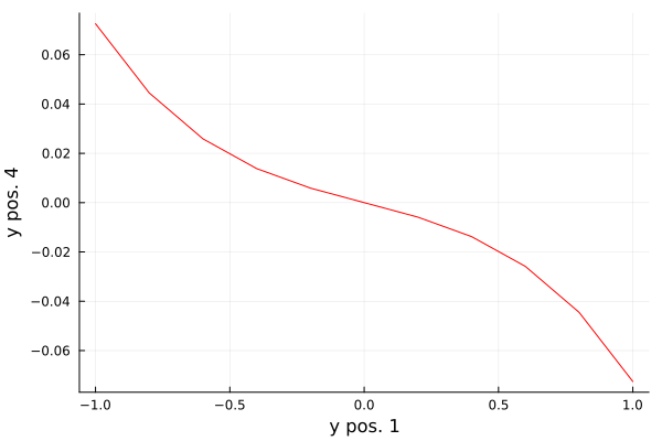
Here is a graph of the dependence of the coordinates of each ray in the beam on the fourth surface (axis Y) from its coordinate on the first surface (axis X).
Team rms_spot returns the RMS scattering of the beam on the last surface of the optical system (if called without additional arguments).
rms = rms_spot( trace1 )
Two-dimensional ray propagation graph
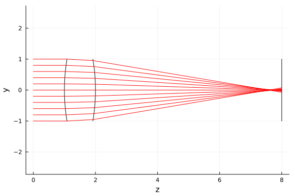
If you pass it to the object optSta not only the characteristics of the source test_bundle, but also an argument rend, then we will get a two-dimensional (or three-dimensional) graph on the output.
p_lens = optSta( test_bundle; rend = "YZ" )
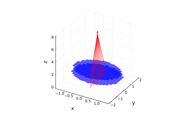
Experiment with the possible arguments of this command to get different graphs (we have converted the graph to the format gr() to speed up rendering).
gr()
rend = "3Dcirc" # @param ["YZ", "XZ", "3Dcirc", "3Dsq"]
ymin = -2.0
ymax = 2.0

p_lens = optSta(test_bundle; rend=rend, ydom = -2:0.1:2)
Conclusion
We learned how to use the library GeometricalOptics to describe simple models that demonstrate the effects of geometric optics (the model does not reflect wave effects).
In addition to installing the library, it took us 7 lines of code to create a model for the propagation of a beam of rays through a lens.