Building a lens model

Let's build a model of an ideal lens using the package GeometricalOptics.jl. We will show how to display several graphs of the propagation of light beams on a single canvas and implement the ray optimization procedure on this graph in order to make the graph the most informative.

Optical system Parameters

To specify the lens parameters, you will need to connect (* and possibly install*) the library GeometricalOptics.

Pkg.add( url="https://github.com/airspaced-nk5/GeometricalOptics.jl#master" )
Pkg.add( "Optim" )

using GeometricalOptics
gr(); # The library works better with this graph rendering mechanism.

Now we can specify several spherical lenses and an image plane.:

Object	Type	Material	Refractive index	Radius R1 (mm)	Radius R2 (mm)	Thickness	Distance to trace.
Lens	biconvex	[SK16](https://refractiveindex.info/?shelf=glass&book ;=HIKARI-SK&page;=SK16)	1.6204	22	430	3	6
Lens	biconcave	[F2](https://refractiveindex.info/?shelf=glass&book ;=SCHOTT-F&page;=F2)	1.6200	22	20	1	6
Lens	biconvex	[SK16](https://refractiveindex.info/?shelf=glass&book ;=HIKARI-SK&page;=SK16)	1.6204	78	16	3	34

The last element of the optical system is the image plane.

The unit of measurement (millimeter) does not play a special role in calculations as long as we do not take into account diffraction and wavelength.

The thickness of the lens is equal to the length of the path that the light ray passes through the lens if it goes along the optical axis.

Radii R1 and R2 are understood as the radius of curvature of each side of each lens: R1 characterizes the radius of curvature of the "input" side located closer to the light source, R2 is the output side of the lens located closer to the image plane.

Let's describe this optical system and build a small visualization.:

surfsList = [ spherical, spherical,
              spherical, spherical,
              spherical, spherical,
              zplane]

p_s = 10; # The distance from the left edge of the graph to the first refractive surface
stations = p_s .+ [ 0., 3., 9., 10., 16., 19., 53. ]
radii = [ 22., -430., -22., 20., 78., -16., 0.0 ]
coeffsList = [ [s, r] for (s,r) in zip(stations, radii)]

# Lens material, in order: SK16, F2, SK16
nList = [ 1., 1.6204,
          1., 1.6200,
          1., 1.6204,
          1.]

optSta = opticalstack( coeffsList, surfsList, nList );

test_bundle = bundle( [0.], (-3:3:3), 0., 0., 0. );
p_lens = optSta( test_bundle; rend = "YZ", halfdomain=3.5 )

plot!( ylimits=(-5,5), aspect_ratio=:none, size=(600,200) )

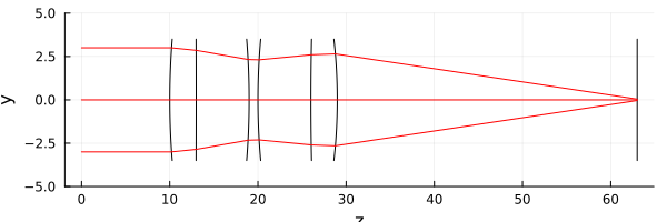
A little visualization allowed us to see all the specified elements.

Aiming the beams at the aperture aperture

Now let's assume that the system has an aperture located 2 mm after the concave lens.

We want to pass beams of light through it, setting a certain angle of incidence, and make sure that they focus on the image plane.

We could split the model into two parts and simulate propagation from the diaphragm in both directions (one model for surfaces [6:end], another for [5:-1:1]). But since the rays should be parallel only when approaching the first lens (* they will not be parallel to each other when passing through the diaphragm*), we would have to look for the angle of each ray when passing through the diaphragm.

Let's go the other way and "optimize" two parameters: the beam width and the point on the Y axis from which the central beam of the beam is directed. Our goal is to find the parameters of a beam whose rays pass exactly through the diaphragm.

angles = [0.0, 0.1, 0.2];             # the angles of each of the beams of rays
colors = [:blue, :green, :red];       # each bundle is characterized by its own color
ypositions_init = [ 0., 3.0, 5.0];    # approximate position of the point of sending the central rays along the Y axis
bundle_halfwidth = 3;                 # the radius of the light beams

p = plot();                           # let's plot a few graphs

for (angle, ypos, pc, plot_surface) in zip(angles, ypositions_init, colors, [true, false, false])
    b = bundle([0.], range(-bundle_halfwidth,bundle_halfwidth,length=3) .- ypos, 0., angle, 0.)
    optSta( b; rend = "YZ", color = pc, plobj = p, halfdomain=5.5, issurfplot=plot_surface )
end

plot!( p, p_s.+[12., 12.], [-2.5, 2.5], lw=2, lc=:black, markershape=:diamond, markercolor=:white );
plot!( p, ylimits=(-8,8), size=(900,400) )

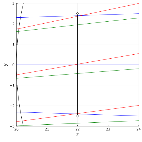
If we zoom in on the image of the aperture, we will see that our first approximation is not very far from the desired one, but for an accurate calculation we need to move the points from where the beams of rays are sent a little.

The beam angle to the optical axis will not change. We are just looking for how to position the beam so that it passes exactly through the diaphragm. This is useful for calculating sensor size and for other interesting results.

plot!( xlimits=(p_s .+ [10, 14]), ylimits=(-3,3), aspect_ratio=:none, size=(500,500) )

Now let's create an optimization procedure.

using Optim

# A new configuration that "ends" with an aperture (although you can add a zplane between any lenses)
optSta2 = opticalstack( [coeffsList[1:4]; [[p_s+12.]]], [surfsList[1:4]; zplane], [nList[1:4] ; 1.0] );

# The function that we will optimize
function f(x, in_angle)
    b_hw = x[1]       # beam radius
    ypos = x[2]       # Y-offset of the beam center
    
    b = bundle([0.], range(-b_hw,b_hw,length=3) .- ypos, 0., in_angle, 0.);
    
    # Let's study the spot at the intersection of the beam with the 6th surface
    t_info = GeometricalOptics.trace_extract_terminus( optSta2( b ), 6, coord="y" );
    
    # Two optimization criteria: both boundaries of the light spot must match the size of the aperture
    q1 = abs( minimum( t_info ) - (-2.5))
    q2 = abs( maximum( t_info ) - ( 2.5)) 
    return q1 + q2
end

angles_hw_list = []
y_positions_list = []
for (angle,y_pos_init) in zip(angles, ypositions_init)
    # We perform optimization for each angle value we need individually.
    res = optimize(x -> f(x, angle), [bundle_halfwidth, y_pos_init])
    angle_optim, ypos_optim = Optim.minimizer( res )
    push!( angles_hw_list, angle_optim )
    push!( y_positions_list, ypos_optim )
end

# Let's display a table of optimization results.
display([["Beam direction"; "Beam width"; "Starting point for Y"] [angles angles_hw_list y_positions_list]'] )

3×4 Matrix{Any}:
 "Направление луча"       0.0         0.1      0.2
 "Ширина пучка"           3.1232      3.13102  3.15749
 "Отправная точка по Y"  -5.40173e-8  2.44082  4.98689

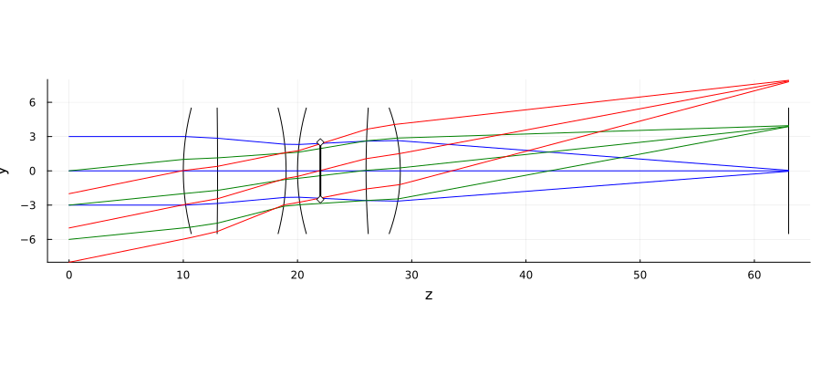
After optimization, the optical system looks like this:

p = plot(); # A canvas for drawing multiple graphs

for (angle, ypos, b_hw, pc, plot_surface) in zip(angles, y_positions_list, angles_hw_list, colors, [true, false, false])
    b = bundle([0.], range(-b_hw,b_hw,length=3) .- ypos, 0., angle, 0.)
    optSta( b; rend = "YZ", color = pc, plobj = p, halfdomain=5.5, issurfplot=plot_surface )
end

plot!( p, p_s.+[12., 12.], [-2.5, 2.5], lw=2, lc=:black, markershape=:diamond, markercolor=:white );
plot!( p, ylimits=(-8,8), size=(900,400) )

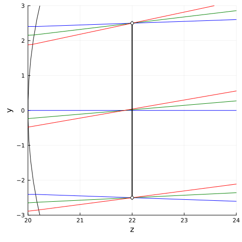
A closer examination of the diaphragm allows you to see the correct position of the light spot.

plot!( xlimits=(p_s .+ [10, 14]), ylimits=(-3,3), aspect_ratio=:none, size=(500,500) )

Lens sizes in the library GeometricalOptics.jl they are not visually taken into account. In some cases, for example, when creating polynomials Цернике, the passage of the beam outside a certain area causes the error provided by the developers.

Conclusion

If you wrap the optical circuit calculation function in an optimization procedure, you can automate many of the optical system design steps. The beams consist of individual rays of light, and their parameters in any section of the system can be obtained using the function trace_extract_terminus and to her подобных.

With the help of a small amount of additional code, it will be possible to calculate the AF range and other tasks.

Data source

[1] Building perfect optics in Zemax [Electronic resource] // Popular science magazine "3D world world" : website. URL: http://mir-3d-world.ipo.spb.ru/2016/3dworld_4_2016.pdf (date of request: 05.11.2024).