Plotting Graphs
TikzGraphs.jl
Another nice graph visualization package. (TikzPictures.jl required to render/save):
julia> g = wheel_graph(10); t = plot(g)

julia> save(SVG("wheel10.svg"), t)
producing a graph like this:

GraphPlot.jl
Another graph visualization package that is very simple to use. Compose.jl is required for most rendering functionality:
julia> using GraphPlot, Compose

julia> g = wheel_graph(10)

julia> draw(PNG("/tmp/wheel10.png", 16cm, 16cm), gplot(g))
NetworkViz.jl
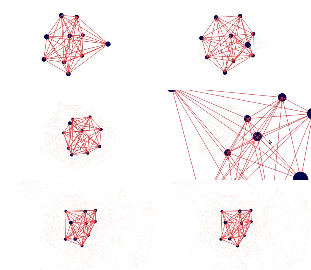
NetworkViz.jl is tightly coupled with LightGraphs.jl. Graphs can be visualized in 2D as well as 3D using ThreeJS.jl and Escher.jl.
#Run this code in Escher

using NetworkViz
using LightGraphs

main(window) = begin
  push!(window.assets, "widgets")
  push!(window.assets,("ThreeJS","threejs"))
  g = complete_graph(10)
  drawGraph(g)
end
The above code produces the following output:

SGtSNEpi.jl
SGtSNEpi.jl is a high-performance software for swift embedding of a large, sparse graph into a d-dimensional space (d = 1,2,3). The Makie plotting ecosystem is used for interactive plots.
using GLMakie, SGtSNEpi, SNAPDatasets

GLMakie.activate!()

g = loadsnap(:as_caida)
y = sgtsnepi(g);
show_embedding(y;
  A = adjacency_matrix(g),        # show edges on embedding
  mrk_size = 1,                   # control node sizes
  lwd_in = 0.01, lwd_out = 0.001, # control edge widths
  edge_alpha = 0.03 )             # control edge transparency
The above code produces the following output:

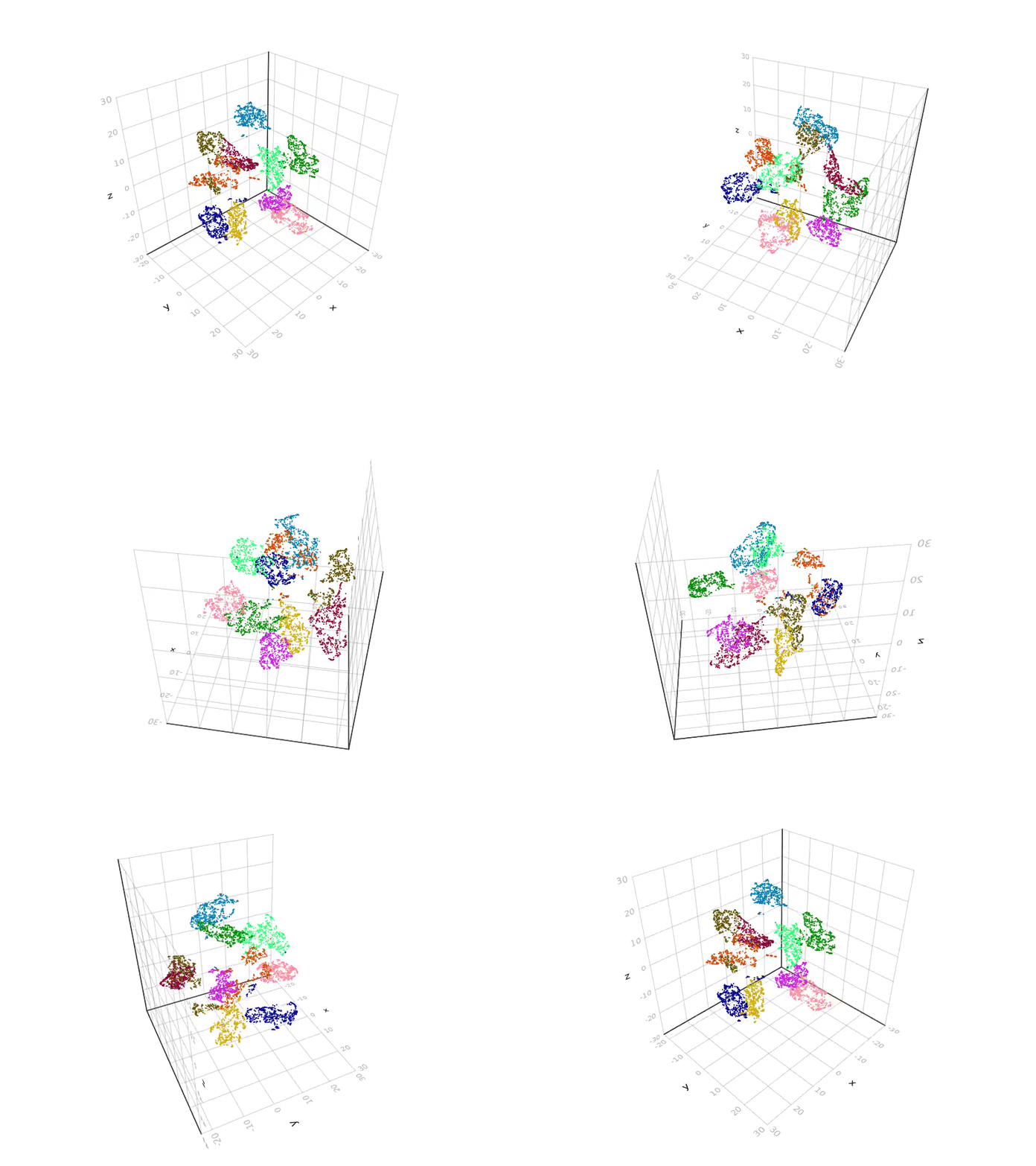
SGtSNEpi.jl enables 3D graph embedding as well. The 3D embedding of the weighted undirected graph ML_Graph/optdigits_10NN is shown below. It consists of 26,475 nodes and 53,381 edges. Nodes are colored according to labels provided with the dataset.

