Examples

Страница в процессе перевода.

These are some basic examples of use of the package:

julia> using Measurements


julia> a = measurement(4.5, 0.1)
4.5 ± 0.1

julia> b = 3.8 ± 0.4
3.8 ± 0.4

julia> 2a + b
12.8 ± 0.45

julia> a - 1.2b
-0.06 ± 0.49

julia> l = measurement(0.936, 1e-3);


julia> T = 1.942 ± 4e-3;


julia> g = 4pi^2*l/T^2
9.798 ± 0.042

julia> c = measurement(4)
4.0 ± 0.0

julia> a*c
18.0 ± 0.4

julia> sind(94 ± 1.2)
0.9976 ± 0.0015

julia> x = 5.48 ± 0.67;


julia> y = 9.36 ± 1.02;


julia> log(2x^2 - 3.4y)
3.34 ± 0.53

julia> atan(y, x)
1.041 ± 0.071

Measurements from Strings

You can construct Measurement{Float64} objects from strings. Within parentheses there is the uncertainty referred to the corresponding last digits.

julia> using Measurements


julia> measurement("-12.34(56)")
-12.34 ± 0.56

julia> measurement("+1234(56)e-2")
12.34 ± 0.56

julia> measurement("123.4e-1 +- 0.056e1")
12.34 ± 0.56

julia> measurement("(-1.234 ± 0.056)e1")
-12.34 ± 0.56

julia> measurement("1234e-2 +/- 0.56e0")
12.34 ± 0.56

julia> measurement("-1234e-2")
-12.34 ± 0.0

It is also possible to use parse(Measurement{T}, string) to parse the string as a Measurement{T}, with T<:AbstractFloat. This has been tested with standard numeric floating types (Float16, Float32, Float64, and BigFloat).

julia> using Measurements


julia> parse(Measurement{Float16}, "19.5 ± 2.8")
19.5 ± 2.8

julia> parse(Measurement{Float32}, "-7.6 ± 0.4")
-7.6 ± 0.4

julia> parse(Measurement{Float64}, "4 ± 1.3")
4.0 ± 1.3

julia> parse(Measurement{BigFloat}, "+5.1 ± 3.3")
5.099999999999999999999999999999999999999999999999999999999999999999999999999986 ± 3.299999999999999999999999999999999999999999999999999999999999999999999999999993

Correlation Between Variables

Here you can see examples of how functionally correlated variables are treated within the package:

julia> using Measurements, SpecialFunctions


julia> x = 8.4 ± 0.7
8.4 ± 0.7

julia> x - x
0.0 ± 0.0

julia> x/x
1.0 ± 0.0

julia> x*x*x - x^3
0.0 ± 0.0

julia> sin(x)/cos(x) - tan(x) # They are equal within numerical accuracy
-2.220446049250313e-16 ± 0.0

julia> y = -5.9 ± 0.2;


julia> beta(x, y) - gamma(x)*gamma(y)/gamma(x + y)
2.8e-14 ± 4.0e-14

You will get similar results for a variable that is a function of an already existing Measurement object:

julia> using Measurements


julia> x = 8.4 ± 0.7;


julia> u = 2x;


julia> (x + x) - u
0.0 ± 0.0

julia> u/2x
1.0 ± 0.0

julia> u^3 - 8x^3
0.0 ± 0.0

julia> cos(x)^2 - (1 + cos(u))/2
0.0 ± 0.0

A variable that has the same nominal value and uncertainty as u above but is not functionally correlated with x will give different outcomes:

julia> using Measurements


julia> x = 8.4 ± 0.7;


julia> v = 16.8 ± 1.4;


julia> (x + x) - v
0.0 ± 2.0

julia> v / 2x
1.0 ± 0.12

julia> v^3 - 8x^3
0.0 ± 1700.0

julia> cos(x)^2 - (1 + cos(v))/2
0.0 ± 0.88

`@uncertain` Macro

Macro @uncertain can be used to propagate uncertainty in arbitrary real or complex functions of real arguments, including functions not natively supported by this package.

julia> using Measurements, SpecialFunctions


julia> @uncertain (x -> complex(zeta(x), exp(eta(x)^2)))(2 ± 0.13)
(1.64 ± 0.12) + (1.967 ± 0.043)im

julia> @uncertain log(9.4 ± 1.3, 58.8 ± 3.7)
1.82 ± 0.12

julia> log(9.4 ± 1.3, 58.8 ± 3.7) # Exact result
1.82 ± 0.12

julia> @uncertain atan(10, 13.5 ± 0.8)
0.638 ± 0.028

julia> atan(10, 13.5 ± 0.8) # Exact result
0.638 ± 0.028

You usually do not need to define a wrapping function before using it. In the case where you have to define a function, like in the first line of previous examples, anonymous functions allow you to do it in a very concise way.

The macro works with functions calling C/Fortran functions as well. For example, Cuba.jl package performs numerical integration by wrapping the C Cuba library. You can define a function to numerically compute with Cuba.jl the integral defining the error function and pass it to @uncertain macro. Compare the result with that of the erf function, natively supported in Measurements.jl package

julia> using Measurements, Cuba, SpecialFunctions
ERROR: ArgumentError: Package Cuba not found in current path.
- Run `import Pkg; Pkg.add("Cuba")` to install the Cuba package.

julia> cubaerf(x::Real) =
           2x/sqrt(pi)*cuhre((t, f) -> f[1] = exp(-abs2(t[1]*x)))[1][1]
cubaerf (generic function with 1 method)

julia> @uncertain cubaerf(0.5 ± 0.01)
ERROR: UndefVarError: `cuhre` not defined

julia> erf(0.5 ± 0.01) # Exact result
ERROR: UndefVarError: `erf` not defined

Also here you can use an anonymous function instead of defining the cubaerf function, do it as an exercise. Remember that if you want to numerically integrate a function that returns a Measurement object you can use QuadGK.jl package, which is written purely in Julia and in addition allows you to set Measurement objects as endpoints, see below.

Note that the argument of @uncertain macro must be a function call. Thus,

julia> using Measurements, SpecialFunctions

julia> @uncertain zeta(13.4 ± 0.8) + eta(8.51 ± 0.67)
ERROR: MethodError: no method matching zeta(::Measurement{Float64})
[...]

will not work because here the outermost function is +, whose arguments are zeta(13.4 ± 0.8) and eta(8.51 ± 0.67), that however cannot be calculated. You can use the @uncertain macro on each function separately:

julia> using Measurements, SpecialFunctions

julia> @uncertain(zeta(13.4 ± 0.8)) +  @uncertain(eta(8.51 ± 0.67))
1.9974 ± 0.0012

In addition, the function must be differentiable in all its arguments. For example, the polygamma function of order , polygamma(m, x), is the -th derivative of the logarithm of gamma function, and is not differentiable in the first argument, because the first argument must be an integer. You can easily work around this limitation by wrapping the function in a single-argument function:

julia> using Measurements, SpecialFunctions

julia> @uncertain (x -> polygamma(0, x))(4.8 ± 0.2)
1.461 ± 0.046

julia> digamma(4.8 ± 0.2)   # Exact result
1.461 ± 0.046

Complex Measurements

Here are a few examples about uncertainty propagation of complex-valued measurements.

julia> using Measurements


julia> u = complex(32.7 ± 1.1, -3.1 ± 0.2);


julia> v = complex(7.6 ± 0.9, 53.2 ± 3.4);


julia> 2u + v
(73.0 ± 2.4) + (47.0 ± 3.4)im

julia> sqrt(u * v)
(33.0 ± 1.1) + (26.0 ± 1.1)im

You can also verify the Euler’s formula

julia> using Measurements


julia> u = complex(32.7 ± 1.1, -3.1 ± 0.2);


julia> cis(u)
(6.3 ± 23.0) + (21.3 ± 8.1)im

julia> cos(u) + sin(u)*im
(6.3 ± 23.0) + (21.3 ± 8.1)im

Missing Measurements

Measurement objects are poisoned by missing values as expected:

julia> using Measurements


julia> x = -34.62 ± 0.93
-34.62 ± 0.93

julia> y = missing ± 1.5
missing

julia> x ^ 2 / y
missing

Arbitrary Precision Calculations

If you performed an exceptionally good experiment that gave you extremely precise results (that is, with very low relative error), you may want to use arbitrary precision (or multiple precision) calculations, in order not to loose significance of the experimental results. Luckily, Julia natively supports this type of arithmetic and so Measurements.jl does. You only have to create Measurement objects with nominal value and uncertainty of type BigFloat.

As explained in the Julia documentation, it is better to use BigFloat("12.34"), rather than BigFloat(12.34). See examples below.

For example, you want to measure a quantity that is the product of two observables and , and the expected value of the product is . You measure and and want to compute the standard score of the product with stdscore. Using the ability of Measurements.jl to perform arbitrary precision calculations you discover that

julia> using Measurements


julia> a = BigFloat("3.00000001") ± BigFloat("1e-17");


julia> b = BigFloat("4.0000000100000001") ± BigFloat("1e-17");


julia> stdscore(a * b, BigFloat("12.00000007"))
7.999999997599999878080000420160000093695993825308195353920411656927305928530607

the measurement significantly differs from the expected value and you make a great discovery. Instead, if you used double precision accuracy, you would have wrongly found that your measurement is consistent with the expected value:

julia> using Measurements


julia> stdscore((3.00000001 ± 1e-17)*(4.0000000100000001 ± 1e-17), 12.00000007)
0.0

and you would have missed an important prize due to the use of an incorrect arithmetic.

Of course, you can perform any mathematical operation supported in Measurements.jl using arbitrary precision arithmetic:

julia> using Measurements


julia> a = BigFloat("3.00000001") ± BigFloat("1e-17");


julia> b = BigFloat("4.0000000100000001") ± BigFloat("1e-17");


julia> hypot(a, b)
5.000000014000000080000000000000000000000000000000000000000000000000000000000013 ± 9.999999999999999999999999999999999999999999999999999999999999999999999999999967e-18

julia> log(2a) ^ b
10.30668110995484998100000000000000000000000000000000000000000000000000000000005 ± 9.699999999999999999999999999999999999999999999999999999999999999999999999999966e-17

Operations with Arrays and Linear Algebra

You can create arrays of Measurement objects and perform mathematical operations on them in the most natural way possible:

julia> using Measurements


julia> A = [1.03 ± 0.14, 2.88 ± 0.35, 5.46 ± 0.97]
3-element Vector{Measurement{Float64}}:
 1.03 ± 0.14
 2.88 ± 0.35
 5.46 ± 0.97

julia> B = [0.92 ± 0.11, 3.14 ± 0.42, 4.67 ± 0.58]
3-element Vector{Measurement{Float64}}:
 0.92 ± 0.11
 3.14 ± 0.42
 4.67 ± 0.58

julia> exp.(sqrt.(B)) .- log.(A)
3-element Vector{Measurement{Float64}}:
 2.58 ± 0.2
 4.82 ± 0.71
  7.0 ± 1.2

julia> @. cos(A) ^ 2 + sin(A) ^ 2
3-element Vector{Measurement{Float64}}:
 1.0 ± 0.0
 1.0 ± 0.0
 1.0 ± 0.0

If you originally have separate arrays of values and uncertainties, you can create an array of Measurement objects using measurement or ± with the dot syntax for vectorizing functions:

julia> using Measurements, Statistics


julia> C = measurement.([174.9, 253.8, 626.3], [12.2, 19.4, 38.5])
3-element Vector{Measurement{Float64}}:
 175.0 ± 12.0
 254.0 ± 19.0
 626.0 ± 38.0

julia> sum(C)
1055.0 ± 45.0

julia> D = [549.4, 672.3, 528.5] .± [7.4, 9.6, 5.2]
3-element Vector{Measurement{Float64}}:
 549.4 ± 7.4
 672.3 ± 9.6
 528.5 ± 5.2

julia> mean(D)
583.4 ± 4.4

prod and sum (and mean, which relies on sum) functions work out-of-the-box with any iterable of Measurement objects, like arrays or tuples. However, these functions have faster methods (quadratic in the number of elements) when operating on an array of Measurement s than on a tuple (in this case the computational complexity is cubic in the number of elements), so you should use an array if performance is crucial for you, in particular for large collections of measurements.

Some linear algebra functions work out-of-the-box, without defining specific methods for them. For example, you can solve linear systems, do matrix multiplication and dot product between vectors, find inverse, determinant, and trace of a matrix, do LU and QR factorization, etc. Additional linear algebra methods (eigvals, cholesky, etc.) are provided by GenericLinearAlgebra.jl.

julia> using Measurements, LinearAlgebra


julia> A = [(14 ± 0.1) (23 ± 0.2); (-12 ± 0.3) (24 ± 0.4)]
2×2 Matrix{Measurement{Float64}}:
  14.0±0.1  23.0±0.2
 -12.0±0.3  24.0±0.4

julia> b = [(7 ± 0.5), (-13 ± 0.6)]
2-element Vector{Measurement{Float64}}:
   7.0 ± 0.5
 -13.0 ± 0.6

julia> x = A \ b
2-element Vector{Measurement{Float64}}:
 0.763 ± 0.031
 -0.16 ± 0.018

julia> A * x ≈ b
true

julia> dot(x, b)
7.42 ± 0.6

julia> det(A)
612.0 ± 9.5

julia> tr(A)
38.0 ± 0.41

julia> A * inv(A) ≈ Matrix{eltype(A)}(I, size(A))
true

julia> lu(A)
LinearAlgebra.LU{Measurement{Float64}, Matrix{Measurement{Float64}}, Vector{Int64}}
L factor:
2×2 Matrix{Measurement{Float64}}:
    1.0±0.0    0.0±0.0
 -0.857±0.022  1.0±0.0
U factor:
2×2 Matrix{Measurement{Float64}}:
 14.0±0.1   23.0±0.2
  0.0±0.0  43.71±0.67

julia> qr(A)
LinearAlgebra.QR{Measurement{Float64}, Matrix{Measurement{Float64}}, Vector{Measurement{Float64}}}
Q factor: 2×2 LinearAlgebra.QRPackedQ{Measurement{Float64}, Matrix{Measurement{Float64}}, Vector{Measurement{Float64}}}
R factor:
2×2 Matrix{Measurement{Float64}}:
 -18.44±0.21  -1.84±0.52
    0.0±0.0   33.19±0.33

Derivative, Gradient and Uncertainty Components

In order to propagate the uncertainties, Measurements.jl keeps track of the partial derivative of an expression with respect to all independent measurements from which the expression comes. The package provides a convenient function, Measurements.derivative, that returns the partial derivative of an expression with respect to independent measurements. Its vectorized version can be used to compute the gradient of an expression with respect to multiple independent measurements.

julia> using Measurements


julia> x = 98.1 ± 12.7
98.0 ± 13.0

julia> y = 105.4 ± 25.6
105.0 ± 26.0

julia> z = 78.3 ± 14.1
78.0 ± 14.0

julia> Measurements.derivative(2x - 4y, x)
2.0

julia> Measurements.derivative(2x - 4y, y)
-4.0

julia> Measurements.derivative.(log1p(x) + y^2 - cos(x/y), [x, y, z])
3-element Vector{Float64}:
   0.017700515090289737
 210.7929173496422
   0.0

The last result shows that the expression does not depend on z.

The vectorized version of Measurements.derivative is useful in order to discover which variable contributes most to the total uncertainty of a given expression, if you want to minimize it. This can be calculated as the Hadamard (element-wise) product between the gradient of the expression with respect to the set of variables and the vector of uncertainties of the same variables in the same order. For example:

julia> w = y^(3//4)*log(y) + 3x - cos(y/x)
447.0410543780643 ± 52.41813324207829

julia> abs.(Measurements.derivative.(w, [x, y]) .* Measurements.uncertainty.([x, y]))
2-element Array{Float64,1}:
 37.9777
 36.1297

In this case, the x variable contributes most to the uncertainty of w. In addition, note that the Euclidean norm of the Hadamard product above is exactly the total uncertainty of the expression:

julia> vecnorm(Measurements.derivative.(w, [x, y]) .* Measurements.uncertainty.([x, y]))
52.41813324207829

The [Measurements.uncertainty_components](usage.md#Measurements.uncertainty_components) function simplifies calculation of all uncertainty components of a derived quantity:

julia> Measurements.uncertainty_components(w)
Dict{Tuple{Float64,Float64,Float64},Float64} with 2 entries:
  (98.1, 12.7, 0.303638)  => 37.9777
  (105.4, 25.6, 0.465695) => 36.1297

julia> norm(collect(values(Measurements.uncertainty_components(w))))
52.41813324207829

`stdscore` Function

You can get the distance in number of standard deviations between a measurement and its expected value (not a Measurement) using stdscore:

julia> using Measurements


julia> stdscore(1.3 ± 0.12, 1)
2.5000000000000004

You can use the same function also to test the consistency of two measurements by computing the standard score between their difference and zero. This is what stdscore does when both arguments are Measurement objects:

julia> using Measurements


julia> stdscore((4.7 ± 0.58) - (5 ± 0.01), 0)
-0.5171645175253433

julia> stdscore(4.7 ± 0.58, 5 ± 0.01)
-0.5171645175253433

`weightedmean` Function

Calculate the weighted and arithmetic means of your set of measurements with weightedmean and mean respectively:

julia> using Measurements, Statistics


julia> weightedmean((3.1±0.32, 3.2±0.38, 3.5±0.61, 3.8±0.25))
3.47 ± 0.17

julia> mean((3.1±0.32, 3.2±0.38, 3.5±0.61, 3.8±0.25))
3.4 ± 0.21

`Measurements.value` and `Measurements.uncertainty` Functions

Use Measurements.value and Measurements.uncertainty to get the values and uncertainties of measurements. They work with real and complex measurements, scalars or arrays:

julia> using Measurements


julia> Measurements.value(94.5 ± 1.6)
94.5

julia> Measurements.uncertainty(94.5 ± 1.6)
1.6

julia> Measurements.value.([complex(87.3 ± 2.9, 64.3 ± 3.0), complex(55.1 ± 2.8, -19.1 ± 4.6)])
2-element Vector{ComplexF64}:
 87.3 + 64.3im
 55.1 - 19.1im

julia> Measurements.uncertainty.([complex(87.3 ± 2.9, 64.3 ± 3.0), complex(55.1 ± 2.8, -19.1 ± 4.6)])
2-element Vector{ComplexF64}:
 2.9 + 3.0im
 2.8 + 4.6im

Calculating the Covariance and Correlation Matrices

Calculate the covariance and correlation matrices of multiple Measurements with the functions Measurements.cov and Measurements.cor:

julia> using Measurements


julia> x = measurement(1.0, 0.1)
1.0 ± 0.1

julia> y = -2x + 10
8.0 ± 0.2

julia> z = -3x
-3.0 ± 0.3

julia> cov([x, y, z])
ERROR: UndefVarError: `cov` not defined

julia> cor([x, y, z])
ERROR: UndefVarError: `cor` not defined

Creating Correlated Measurements from their Nominal Values and a Covariance Matrix

Using Measurements.correlated_values, you can correlate the uncertainty of fit parameters given a covariance matrix from the fitted results. An example using LsqFit.jl:

julia> using Measurements, LsqFit


julia> @. model(x, p) = p[1] + x * p[2]
model (generic function with 1 method)

julia> xdata = range(0, stop=10, length=20)
0.0:0.5263157894736842:10.0

julia> ydata = model(xdata, [1.0 2.0]) .+ 0.01 .* randn.()
20-element Vector{Float64}:
  1.00290802497355
  2.057933169002546
  3.0930244217442944
  4.174794200214189
  5.19684307772886
  6.250257118205858
  7.30382236891682
  8.369018710257013
  9.428192303550444
 10.480817953638747
 11.521575448459055
 12.589452224466132
 13.6427575489115
 14.668798221177974
 15.74105892180237
 16.81242399070085
 17.840821380682414
 18.884270129715922
 19.94514569695481
 21.008574360349133

julia> p0 = [0.5, 0.5]
2-element Vector{Float64}:
 0.5
 0.5

julia> fit = curve_fit(model, xdata, ydata, p0)
LsqFit.LsqFitResult{Vector{Float64}, Vector{Float64}, Matrix{Float64}, Vector{Float64}, Vector{LsqFit.LMState{LsqFit.LevenbergMarquardt}}}([0.9980960278243373, 2.000505687149637], [-0.0048119971492127656, -0.006939411099452286, 0.010867066237555623, -0.018004982153581928, 0.012843870410502944, 0.01232756001226143, 0.011660039380055665, -0.0006385718813799457, -0.006914435096055271, -0.006642355105601183, 0.00549788015284669, -0.00948116577547431, -0.009888760142086284, 0.016968297670196364, -0.002394672875443149, -0.020862011695168547, 0.0036383284020260476, 0.013087309447271878, 0.00510947228714187, -0.005421461028422669], [1.0000000000052196 0.0; 1.0000000000235538 0.5263157894859544; … ; 1.0000000000235538 9.473684210527223; 1.0000000000235538 9.9999999999032], true, Iter     Function value   Gradient norm
------   --------------   --------------
, Float64[])

julia> coeficients = Measurements.correlated_values(coef(fit), estimate_covar(fit))
2-element Vector{Measurement{Float64}}:
  0.9981 ± 0.0048
 2.00051 ± 0.00082

julia> f(x) = model(x, coeficients)
f (generic function with 1 method)

Interplay with Third-Party Packages

Measurements.jl works out-of-the-box with any function taking arguments no more specific than AbstractFloat. This makes this library particularly suitable for cooperating with well-designed third-party packages in order to perform complicated calculations always accurately taking care of uncertainties and their correlations, with no effort for the developers nor users.

The following sections present a sample of packages that are known to work with Measurements.jl, but many others will interplay with this package as well as them.

Numerical Integration with `QuadGK.jl`

The powerful integration routine quadgk from QuadGK.jl package is smart enough to support out-of-the-box integrand functions that return arbitrary types, including Measurement:

julia> using Measurements, QuadGK
ERROR: ArgumentError: Package QuadGK not found in current path.
- Run `import Pkg; Pkg.add("QuadGK")` to install the QuadGK package.

julia> a = 4.71 ± 0.01;


julia> quadgk(x -> exp(x / a), 1, 7)[1]
ERROR: UndefVarError: `quadgk` not defined

You can also use Measurement objects as endpoints:

julia> using Measurements, QuadGK
ERROR: ArgumentError: Package QuadGK not found in current path.
- Run `import Pkg; Pkg.add("QuadGK")` to install the QuadGK package.

julia> quadgk(cos, 1.19 ± 0.02, 8.37 ± 0.05)[1]
ERROR: UndefVarError: `quadgk` not defined

Compare this with the expected result:

julia> using Measurements


julia> sin(8.37 ± 0.05) - sin(1.19 ± 0.02)
-0.059 ± 0.026

Also with quadgk correlation is properly taken into account:

julia> using Measurements, QuadGK
ERROR: ArgumentError: Package QuadGK not found in current path.
- Run `import Pkg; Pkg.add("QuadGK")` to install the QuadGK package.

julia> a = 6.42 ± 0.03
6.42 ± 0.03

julia> quadgk(sin, -a, a)[1]
ERROR: UndefVarError: `quadgk` not defined

The uncertainty of the result is compatible with zero, within the accuracy of double-precision floating point numbers. If instead the two endpoints have, by chance, the same nominal value and uncertainty but are not correlated the uncertainty of the result is non-zero:

julia> using Measurements, QuadGK
ERROR: ArgumentError: Package QuadGK not found in current path.
- Run `import Pkg; Pkg.add("QuadGK")` to install the QuadGK package.

julia> quadgk(sin, -6.42 ± 0.03, 6.42 ± 0.03)[1]
ERROR: UndefVarError: `quadgk` not defined

Numerical and Automatic Differentiation

With Calculus.jl package it is possible to perform numerical differentiation using finite differencing. You can pass in to the Calculus.derivative function both functions returning Measurement objects and a Measurement as the point in which to calculate the derivative.

julia> using Measurements, Calculus
ERROR: ArgumentError: Package Calculus not found in current path.
- Run `import Pkg; Pkg.add("Calculus")` to install the Calculus package.

julia> a = -45.7 ± 1.6
-45.7 ± 1.6

julia> b = 36.5 ± 6.0
36.5 ± 6.0

julia> Calculus.derivative(exp, a) ≈ exp(a)
ERROR: UndefVarError: `Calculus` not defined

julia> Calculus.derivative(cos, b) ≈ -sin(b)
ERROR: UndefVarError: `Calculus` not defined

julia> Calculus.derivative(t -> log(-t * b) ^ 2, a) ≈ 2 * log(-a * b) / a
ERROR: UndefVarError: `Calculus` not defined

Other packages provide automatic differentiation methods. Here is an example with AutoGrad.jl, just one of the packages available:

julia> using Measurements, AutoGrad
ERROR: ArgumentError: Package AutoGrad not found in current path.
- Run `import Pkg; Pkg.add("AutoGrad")` to install the AutoGrad package.

julia> a = -45.7 ± 1.6
-45.7 ± 1.6

julia> b = 36.5 ± 6.0
36.5 ± 6.0

julia> grad(exp)(a) ≈ exp(a)
ERROR: UndefVarError: `grad` not defined

julia> grad(cos)(b) ≈ -sin(b)
ERROR: UndefVarError: `grad` not defined

julia> grad(t -> log(-t * b) ^ 2)(a) ≈ 2 * log(-a * b) / a
ERROR: UndefVarError: `grad` not defined

However remember that you can always use Measurements.derivative to compute the value (without uncertainty) of the derivative of a Measurement object.

Use with `Unitful.jl`

You can use Measurements.jl in combination with Unitful.jl in order to perform calculations involving physical measurements, i.e. numbers with uncertainty and physical unit. You only have to use the Measurement object as the value of the Quantity object. Here are a few examples.

julia> using Measurements, Unitful
ERROR: ArgumentError: Package Unitful not found in current path.
- Run `import Pkg; Pkg.add("Unitful")` to install the Unitful package.

julia> hypot((3 ± 1)*u"m", (4 ± 2)*u"m") # Pythagorean theorem
ERROR: LoadError: UndefVarError: `@u_str` not defined
in expression starting at REPL[2]:1

julia> (50 ± 1)*u"Ω" * (13 ± 2.4)*1e-2*u"A" # Ohm's Law
ERROR: LoadError: UndefVarError: `@u_str` not defined
in expression starting at REPL[3]:1

julia> 2pi*sqrt((5.4 ± 0.3)*u"m" / ((9.81 ± 0.01)*u"m/s^2")) # Pendulum's period
ERROR: LoadError: UndefVarError: `@u_str` not defined
in expression starting at REPL[4]:1

Integration with `Plots.jl`

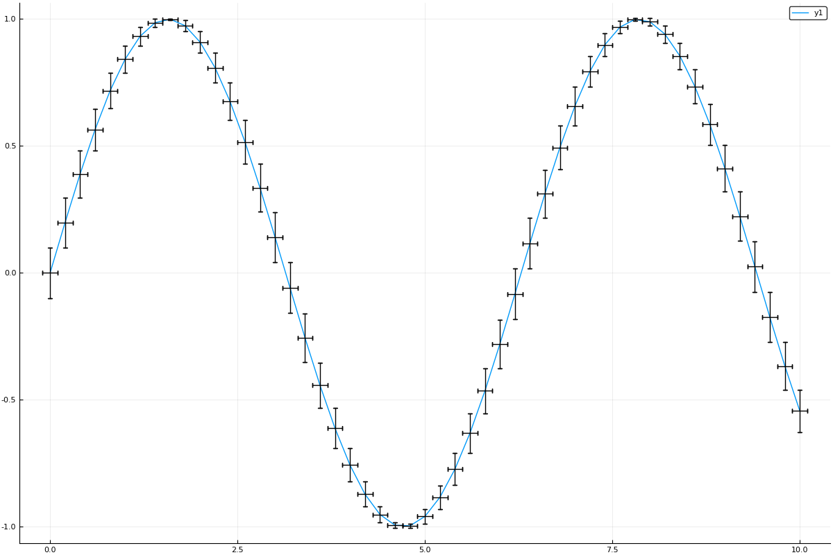
Measurements.jl provides plot recipes for the Julia graphic framework Plots.jl. Arguments to plot function that have Measurement type will be automatically represented with errorbars.

julia> using Measurements, Plots

julia> plot(sin, [x ± 0.1 for x in 1:0.2:10], size = (1200, 800))

Examples

Measurements from Strings

Correlation Between Variables

@uncertain Macro

Complex Measurements

Missing Measurements

Arbitrary Precision Calculations

Operations with Arrays and Linear Algebra

Derivative, Gradient and Uncertainty Components

stdscore Function

weightedmean Function

Measurements.value and Measurements.uncertainty Functions

Calculating the Covariance and Correlation Matrices

Creating Correlated Measurements from their Nominal Values and a Covariance Matrix

Interplay with Third-Party Packages

Numerical Integration with QuadGK.jl

Numerical and Automatic Differentiation

Use with Unitful.jl

Integration with Plots.jl

`@uncertain` Macro

`stdscore` Function

`weightedmean` Function

`Measurements.value` and `Measurements.uncertainty` Functions

Numerical Integration with `QuadGK.jl`

Use with `Unitful.jl`

Integration with `Plots.jl`