lsqnonlin
|
Page in progress. |
A solver of nonlinear least squares problems.
| Library |
|
Description
Function lsqnonlin solves the nonlinear least squares problem of the form:
where
The function is called when solving an optimization problem. optimize or creating optimization settings OptimizeOptions.
Solver Settings
| All algorithms | |||
|---|---|---|---|
|
Choose one of the algorithms: Argument |
||
|
Display diagnostic information about the function to be minimized or solved. Available options: |
||
|
The maximum change in variables for finite difference gradients (positive scalar). Default value — |
||
|
Minimal change of variables for finite difference gradients (positive scalar). Default value — |
||
|
Output level:
|
||
|
Scalar or vector step size coefficient for the finite difference method. If the argument is where Scalar value |
||
|
The final differences used to estimate gradients can be When evaluating both types of finite differences, the algorithm strictly adheres to the specified boundaries. For example, instead of a direct difference, the inverse can be used to avoid calculating the function at a point outside the acceptable range. |
||
|
Tolerance for the value of the function to terminate the algorithm; non-negative scalar. Default value — |
||
|
Checking the correctness of function values. When choosing |
||
|
The maximum allowed number of calculations of the function, set as a non-negative integer. The default value is |
||
|
The maximum allowed number of iterations, set as a non-negative integer. The default value is |
||
|
The tolerance for the stopping condition according to the optimality criterion of the first order, given as a non-negative scalar. Default value — Algorithm |
||
|
Specify one or more custom functions that the optimization function will call at each iteration. Pass a pointer to a function or an array with function pointers. By default, there are no functions ( |
||
|
Plotting various graphs reflecting the progress of the algorithm; you can select ready-made graphs or create your own. The argument is passed a name, a pointer to a function, or an array containing names or pointers to functions. For custom charting functions, pointers to functions should be passed. By default, charting is disabled (value Custom charting functions use the same syntax as the output functions. |
||
|
If the value is set to |
||
|
Variable tolerance , set as a non-negative scalar, to terminate the algorithm. The default value is |
||
|
Typical values . The number of items in |
||
|
Option for using parallel computing to estimate gradients, set to one of the following values:
|
||
Algorithm |
|||
|
The multiplication function by the Jacobi matrix, specified as a pointer to the function. For large-scale problems with a special structure, this function computes the product where Function
In all cases, the matrix
|
||
|
The Jacobian sparsity pattern for the finite difference method. Install Use If the structure of the matrix is unknown, do not specify |
||
|
Defines the method for calculating the iteration step. When using the default option ( |
||
Algorithm |
|||
|
The initial value of the Levenberg—Marquardt parameter is a positive scalar. Default value — |
||
|
Meaning |
||
Information output by the solver
# resnorm — the square of the discrepancy norm
+
a non-negative real number
Details
The square of the discrepancy norm, returned as a non-negative real number. resnorm — this is the square of the second norm of the discrepancy at the point : .
# residual — the value of the objective function at the solution point
+
array
Details
The value of the objective function at the solution point, returned as an array. In the general case: .
# exitflag — the reason for stopping the solver
+
an integer
Details
The reason for stopping the solver, returned as an integer.
| Meaning | Reason |
|---|---|
|
The function has converged to a solution . |
|
Change less than the specified tolerance, or the Jacobian at the point not defined. |
|
The discrepancy change is less than the specified tolerance. |
|
The relative magnitude of the search direction is less than the tolerance by a step. |
|
The number of iterations exceeded the value |
|
The plotting function or the output function has stopped the solver. |
|
A valid point was not found. The borders and are contradictory, or the solver stopped at an invalid point. |
# output — information about the optimization process
+
structure
Details
Information about the optimization process returned as a structure with fields:
| Field Name | Content |
|---|---|
|
A measure of optimality of the first order. |
|
The number of iterations performed. |
|
The number of calculations of the function. |
|
Total number of iterations of the conjugate gradient method (PCG) (for the algorithm |
|
The final offset in |
|
The optimization algorithm used. |
|
Exit message. |
# lambda — Lagrange multipliers at the solution point
+
structure
Details
Lagrange multipliers at the solution point, returned as a structure with fields:
| Field Name | Content |
|---|---|
|
Lower bounds corresponding to . |
|
Upper bounds corresponding to . |
# jacobian — the Jacobian at the decision point
+
the real matrix
Details
The Jacobian at the solution point, returned as a real matrix. Element jacobian(i,j) It is a partial derivative of a function by variable at the decision point .
For problems in which there are active constraints at the solution point, the Jacobian is not suitable for estimating confidence intervals.
Additional Info
Local and global minimum
Details
A local minimum of a function is a point at which the value of the function is less than at neighboring points, but possibly greater than at any remote point.
The global minimum is the point at which the value of the function is less than at all other acceptable points.
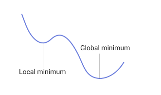
Solver algorithms try to find a local minimum. The result may be a global minimum.
A measure of optimality of the first order
Details
For unconditional optimization problems, the measure of optimality of the first order is the maximum absolute value of the components of the gradient vector (also called the infinite gradient norm). At the minimum point, this value should be zero.
For problems with constraints, the measure of optimality of the first order is the maximum in the index. values . Here — -I am a component of the gradient, — the current point, and
If If it is located on the border, then it is equal to zero. If If it is not located on the border, then at the minimum point the gradient must be equal to zero. Therefore, at the point of the minimum, the measure of optimality of the first order should be zero.
Tolerances
Details
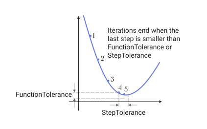
As a rule, tolerance is a threshold value, at which the iterative process of the solver stops.
-
OptimalityTolerance— defines the acceptable deviation for the measure of optimality of the first order. The iterative process ends when the value of the first-order optimality measure becomes less thanOptimalityTolerance. -
FunctionTolerance— determines the amount of the last change in the value of the objective function.
The magnitude of the gradient
Details
The gradient vector is the gradient of the sum of squares. For unconditional optimization problems, the gradient value is considered to be the maximum absolute value of the components of the gradient vector (also called the infinite gradient norm). At the minimum point, this value should be zero.
For problems with constraints, the gradient value is defined as the maximum by the index values . Here — -I am a component of the gradient, — the current point, and
If If it is located on the border, then it is equal to zero. If If it is not on the border, then at the minimum point the gradient must be equal to zero. Therefore, the gradient value should be zero at the minimum point.
Current step size
Details
The size of the current step is the amount of change in the position of the current point in the last iteration.
The local singularity
Details
The Levenberg—Marquardt regularization parameter is related to the inverse of the radius of the confidence region. It takes on large values when the sum of the squares of the function values differs significantly from the quadratic model.
When calculating the Jacobian is impossible
Details
The algorithms evaluate the Jacobian of the target vector function using the finite difference method. If, during the calculation of the final difference, the calculated point has gone beyond the area where the objective function is defined correctly, then this can lead to Inf, NaN or a complex number.
Algorithms
The Levenberg—Marquardt methods and the confidence region with reflection are based on algorithms of the nonlinear least squares method.
-
The default reflection confidence region algorithm is a subspace confidence region method and is based on Newton’s method with internal reflection described in [1] and [2]. Each iteration includes an approximate solution of a large linear system using the preconditioned conjugate gradients (PCG) method.
-
The Levenberg—Marquardt method is described in [4], [5] and [6].
Literature
-
Coleman, T.F. and Y. Li. An Interior, Trust Region Approach for Nonlinear Minimization Subject to Bounds. SIAM Journal on Optimization, Vol. 6, 1996, pp. 418–445.
-
Coleman, T.F. and Y. Li. On the Convergence of Reflective Newton Methods for Large-Scale Nonlinear Minimization Subject to Bounds. Mathematical Programming, Vol. 67, Number 2, 1994, pp. 189–224.
-
Dennis, J. E. Jr. Nonlinear Least-Squares. State of the Art in Numerical Analysis, ed. D. Jacobs, Academic Press, pp. 269–312.
-
Levenberg, K. A Method for the Solution of Certain Problems in Least-Squares. Quarterly Applied Mathematics 2, 1944, pp. 164–168.
-
Marquardt, D. An Algorithm for Least-squares Estimation of Nonlinear Parameters. SIAM Journal Applied Mathematics, Vol. 11, 1963, pp. 431–441.
-
Moré, J. J. The Levenberg-Marquardt Algorithm: Implementation and Theory. Numerical Analysis, ed. G. A. Watson, Lecture Notes in Mathematics 630, Springer Verlag, 1977, pp. 105–116.
-
Moré, J. J., B. S. Garbow, and K. E. Hillstrom. User Guide for MINPACK 1. Argonne National Laboratory, Rept. ANL–80–74, 1980.
-
Powell, M. J. D. A Fortran Subroutine for Solving Systems of Nonlinear Algebraic Equations. Numerical Methods for Nonlinear Algebraic Equations, P. Rabinowitz, ed., Ch.7, 1970.