Frequency analysis of autonomic heart rate control
Note
In this example, the term "vagal activity" is used as a synonym for "vagal activity" (from Nervus vagus - vagus nerve) and means the activity of the parasympathetic branch of the autonomic nervous system.
List of abbreviations used
BP - Blood pressure
DSA - Respiratory sinus arrhythmia
LFM - Linear frequency modulated
SA - Sinoatrial
Low-pass low-pass filter
HR - Heart rate
ABP - Arterial blood pressure
HR - Heart rate
RSA - Respiratory sinus arrhythmia
Additional functions
using EngeeDSP
To run the model, use the additional function run_model.
# Function for launching the model
function run_model( name_model, path_to_folder )                # Defining a function for running the model
    Path = path_to_folder * "/" * name_model * ".engee"
    if name_model in [m.name for m in engee.get_all_models()]   # Checking the condition for loading a model into the kernel
        model = engee.open( name_model )                        # Open the model
        model_output = engee.run( model, verbose=true );        # Launch the model
        engee.close( name_model, force=true );                  # Close the model
    else
        model = engee.load( Path, force=true )                  # Upload a model
        model_output = engee.run( model, verbose=true );        # Launch the model
        engee.close( name_model, force=true );                  # Close the model
    end
    return model_output
end;
For frequency analysis of the results, we will use the freq_analysis function.
function freq_analysis(V, HR, Fs)
    n = length(V)

    # Application of the Hannah window
    window = EngeeDSP.Functions.hann(n)
    V_win = V .* window
    HR_win = HR .* window

    # FFT Calculation
    fft_V = EngeeDSP.rfft(V_win) / n
    fft_HR = EngeeDSP.rfft(HR_win) / n
    freq = EngeeDSP.rfftfreq(n, Fs)

    # Mutual spectrum
    power_V = abs2.(fft_V) * (n / sum(window.^2))
    cross_power = fft_HR .* conj(fft_V) * (n / sum(window.^2))

    # Transfer function
    H = @. cross_power / (power_V + eps())
    amplitude = abs.(H)
    phase_deg = EngeeDSP.rad2deg.(EngeeDSP.angle.(H))

    # Limit to 0.3 Hz
    max_index = findlast(f -> f <= 0.3, freq)  # Finding the last index with a frequency <= 0.3 Hz
    freq = freq[1:max_index]
    amplitude = amplitude[1:max_index]
    phase_deg = phase_deg[1:max_index]

    return amplitude, phase_deg, freq
end;
Introduction
Short-term regulation of heart rate (HR) and blood pressure (BP) is mainly carried out due to feedback through arterial baroceptors, both parameters are constantly influenced by breathing. Breathing affects the heart and blood vessels in several interconnected ways. Changes in pressure inside the chest during inhalation and exhalation directly affect the amount of blood pressure; these fluctuations in blood pressure, in turn, change the heart rate through baroreceptor reflexes. In addition, modern research shows that the respiratory center in the medulla oblongata has direct neural connections with the autonomic centers that control the work of the heart. The cumulative result of this complex effect of breathing is manifested in the form of respiratory sinus arrhythmia (TSA), a natural phenomenon in which the heartbeat accelerates slightly on inspiration and slows down on exhalation. The strength of this effect of breathing on heart rate (DSA value) can be quantified using a special mathematical analysis – the frequency transfer function. Changes in the characteristics of this analysis (for example, a phase shift or a change in amplitude) serve as an indicator of changes in the work of the autonomic nervous system, which regulates the heart rate.
The implementation of the blood circulation model ("Blood_circulation.engee") is shown in the figure below.
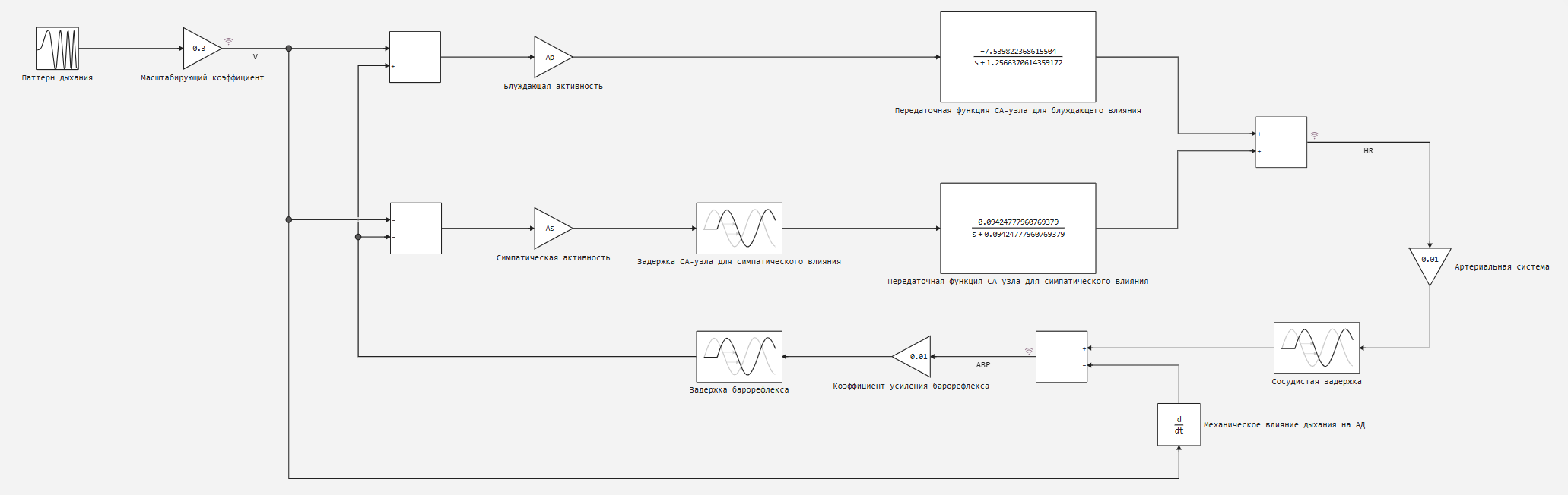
Respiration, measured as a change in lung volume (V), is assumed to have a direct effect on the autonomic inputs of the sinoatrial node (CA node): inhalation leads to a decrease in both vagal and sympathetic efferent activity. Feedback from baroreceptors also directly affects the autonomic inputs of the heart: an increase in blood pressure (ABP) causes a decrease in sympathetic activity and an increase in parasympathetic (vagus) activity.
During inspiration, a decrease in vagal efferent activity acts on the CA node, increasing heart rate (HR). The transfer function simulating the dynamics of this ratio (the wandering branch) is a simple low-pass filter with a cutoff frequency (fp) and a negative gain (-Kp). On the contrary, the response of the CA node to sympathetic stimulation is much slower. In addition to a delay of 1-2 seconds, the transfer function describing the dynamics of the conversion of sympathetic activity into heart rate has a cutoff frequency (fs). In this case, the gain is positive. Heart rate changes are assumed to affect blood pressure after a delay of 0.42 seconds. For simplicity, the transfer function representing the properties of the arterial vascular bed is considered static with a gain of 0.01. In addition, since the conversion of BP (ABP) into the output signal of baroreceptors occurs with very fast dynamics, it is assumed that the baroreflex can be represented by a static gain of 0.01, switched on sequentially with a fixed delay of 0.3 s. Also, direct mechanical The effect of breathing on blood pressure (ABP) is modeled as a negative differentiator, that is, inhalation tends to lower blood pressure (ABP), and exhalation tends to increase it. Thus, the model simulates respiratory sinus arrhythmia by allowing direct autonomic stimulation of heart rate (HR). In addition, the resulting changes in heart rate (HR) and the direct mechanical effect of breathing cause fluctuations in blood pressure (ABP), which subsequently affect heart rate (HR) through baroreflections.
Simulation of the blood circulation model
Initialization of simulation parameters
A linear frequency modulated signal generator will be used to determine the frequency response of the human circulatory model. In this example, the parameters will be set so that the initial frequency is 0.005 Hz and the target frequency is 0.5 Hz. Since the amplitude of the LFM signal generator unit does not change, it is necessary to use a gain factor of 0.3, which limits the amplitude range to 0.6 liters.
Ts = 10e-3               # Step size, with
time_simulation = 300    # Simulation time, with

# Respiratory Pattern Parameters (Chirp)
target_time = 300       # Target time, from
freq_initial = 0.005    # Initial frequency, Hz
freq_target = 0.5;      # Target frequency, Hz
Time delays in accordance with physiological parameters.
time_delay_sym = 2      # CA node delay for sympathetic influence, with
time_delay_vas = 0.42   # Vascular delay, with
time_delay_bar = 0.3;   # Baroreflex delay, s
The following nominal values of the parameters represent a healthy subject in a supine position:
-
Gain of the transfer function of the CA node for the wandering influence, Kp = 6;
-
Gain of the transfer function of the CA node for sympathetic influence Ks = 18;
-
The cutoff frequency of the CA node transfer function for the wandering influence, fp = 0.2 Hz;
-
Cutoff frequency of the CA node transfer function for sympathetic influence, fs = 0.015 Hz;
-
The weighting factors for converting respiratory drive into efferent nervous activity are:
-
For a wandering branch: Ap = 2.5,
-
For the sympathetic branch: As = 0.4.
-
Kp = 6      # Coefficient of amplification of the transfer function of the CA node for the wandering influence
Ks = 18     # The coefficient of amplification of the transfer function of the CA node for sympathetic influence
Ap = 2.5    # Weight factor for a wandering branch
As = 0.4    # Weight factor for the sympathetic branch
fp = 0.2    # Frequency of the cutoff of the transfer function of the CA node for the wandering influence, Hz
fs = 0.015; # Frequency of the cutoff of the transfer function of the CA node for sympathetic influence, Hz
Launching the model
Let's start calculating the simulation of the model using the run_model function.
out = run_model("Blood_circulation", @__DIR__); # Launching the model
Extraction of the obtained results.
V_normal= out["V"].value;
HR_normal = out["HR"].value;
ABP_normal = out["ABP"].value;

time_steps= length(V_normal)
time_model = range(0, step=Ts, length=time_steps);
Visualization of simulation results
The figure below shows the simulation results, and the first 200 seconds of the simulation are presented for greater clarity. The upper graph shows the breathing pattern, that is, the FM signal generator. The average graph corresponds to a change in heart rate. Note that at low frequencies, the heart rate fluctuates almost synchronously with the change in lung volume; however, at higher frequencies, it begins to lag relative to breathing. In addition, the amplitude of the HR signal decreases with increasing frequency, emphasizing the nature of the overall frequency response of the filter. The lower graph shows the change in blood pressure. It can be noted that as the frequency increases, the respiratory-induced changes in blood pressure (ABP) become greater. This is a consequence of the increasing influence of direct mechanical effects of respiration with increasing frequency.
# Visualization of results
max_time = 200      # Time according to OH, with

plot(
    # Volume graph (V)
    plot(time_model, V_normal;
         xlabel="Time, from",
         ylabel="Volume, l",
         label="Change in lung volume (V)",
         legend=:topright,
         linewidth=1.5,
         color=:blue,
         grid=true,
         xlims=(0, max_time),
         ylims=(-0.4, 0.4)),

    # Heart Rate Chart (HR)
    plot(time_model, HR_normal;
         xlabel="Time, from",
         ylabel="Heart rate, beats/min",
         label=" Change in heart rate (HR)",
         legend=:topright,
         linewidth=1.5,
         color=:red,
         grid=true,
         xlims=(0, max_time),
         ylims=(-10, 10)),

    # Blood Pressure Chart (ABP)
    plot(time_model, ABP_normal;
         xlabel="Time, from",
         ylabel="Pressure, mmHg",
         label="Change in blood pressure (ABP)",
         legend=:topright,
         linewidth=1.5,
         color=:green,
         grid=true,
         xlims=(0, max_time),
         ylims=(-1, 1)),

    # General settings for the entire chart
    layout = (3, 1),
    size = (1500, 1000),
    margin = 40 * Plots.px,
    plot_title = "Physiological indicators"
)
Frequency response
Fs = 1 / Ts

# Calculation of frequency characteristics
amplitude_normal, phase_deg_normal, freq_normal = freq_analysis(V_normal,HR_normal, Fs)

plot(
    plot(freq_normal, amplitude_normal;
         title = "Amplitude-frequency response",
         xlabel = "Frequency, Hz",
         ylabel = "|H|, min/l",
         legend = false,
         label = false,
         linewidth = 2.5,
         color = :blue,
         grid = true,
        xlims = (0, 0.3)),

    plot(freq_normal, phase_deg_normal;
         title = "Phase frequency response",
         xlabel = "Frequency, Hz",
         ylabel = "Phase, °",
         legend = false,
         label = false,
         linewidth = 2.5,
         color = :red,
         grid = true,
         ylims = (-180, 180),
         xlims = (0, 0.3)),

    layout = (2, 1),
    size = (1500, 1000),
    margin = 40*Plots.px,
    plot_title = "Transfer function analysis: V → HR"
)
Imitation of drug administration
In this part, two scenarios will be considered that take into account the effect of drugs on the studied parameters.
The first scenario
This scenario simulates the administration of a dose of atropine. This drug causes complete parasympathetic (vagal) blockade. In addition, the model parameters were changed to simulate a situation when the patient is in a standing position, when the sympathetic effect on heart rate increases. Under such conditions, heart rate control would be modulated primarily by the sympathetic nervous system.
Initializing the parameters for the first scenario
The values of the model parameters used to simulate the administration of an atropine dose are presented below:
Kp = 1      # Coefficient of amplification of the transfer function of the CA node for the wandering influence
Ks = 9      # The coefficient of amplification of the transfer function of the CA node for sympathetic influence
Ap = 0.1    # Weight factor for a wandering branch
As = 4      # Weight factor for the sympathetic branch
fp = 0.07   # Frequency of the cutoff of the transfer function of the CA node for the wandering influence, Hz
fs = 0.015; # Frequency of the cutoff of the transfer function of the CA node for sympathetic influence, Hz
Launching the model
out_atropine = run_model("Blood_circulation", @__DIR__); # Launching the model
V_atropine= out_atropine["V"].value;
HR_atropine = out_atropine["HR"].value;
ABP_atropine = out_atropine["ABP"].value;
Visualization of the simulation results of the first scenario
# Visualization of results
max_time = 200      # Time according to OH, with

plot(
    # Volume graph (V)
    plot(time_model, V_atropine;
         xlabel="Time, from",
         ylabel="Volume, l",
         label="Change in lung volume (V)",
         legend=:topright,
         linewidth=1.5,
         color=:blue,
         grid=true,
         xlims=(0, max_time),
         ylims=(-0.4, 0.4)),

    # Heart Rate Chart (HR)
    plot(time_model, HR_atropine;
         xlabel="Time, from",
         ylabel="Heart rate, beats/min",
         label=" Change in heart rate (HR)",
         legend=:topright,
         linewidth=1.5,
         color=:red,
         grid=true,
         xlims=(0, max_time),
         ylims=(-10, 10)),

    # Blood Pressure Chart (ABP)
    plot(time_model, ABP_atropine;
         xlabel="Time, from",
         ylabel="Pressure, mmHg",
         label="Change in blood pressure (ABP)",
         legend=:topright,
         linewidth=1.5,
         color=:green,
         grid=true,
         xlims=(0, max_time),
         ylims=(-1, 1)),

    # General settings for the entire chart
    layout = (3, 1),
    size = (1500, 1000),
    margin = 40 * Plots.px,
    plot_title = "Physiological parameters during the administration of atropine"
)
# Calculation of frequency characteristics
amplitude_atropine, phase_deg_atropine, freq_atropine = freq_analysis(V_atropine,HR_atropine, Fs)

plot(
    plot(freq_atropine, amplitude_atropine;
         title = "Amplitude-frequency response",
         xlabel = "Frequency, Hz",
         ylabel = "|H|, min/l",
         legend = false,
         label = false,
         linewidth = 2.5,
         color = :blue,
         grid = true,
         xlims = (0, 0.3)),

    plot(freq_atropine, phase_deg_atropine;
         title = "Phase frequency response",
         xlabel = "Frequency, Hz",
         ylabel = "Phase, °",
         legend = false,
         label = false,
         linewidth = 2.5,
         color = :red,
         grid = true,
         ylims = (-180, 180),
         xlims = (0, 0.3)),

    layout = (2, 1),
    size = (1200, 1000),
    margin = 40*Plots.px,
    plot_title = "Transfer function analysis: V → HR"
)
The second scenario
This scenario simulates the administration of a dose of propranolol. This drug causes beta-adrenergic blockade. In addition, we assume a supine position, which makes wandering modulation the predominant control mode.
Initializing the parameters for the second scenario
The values of the model parameters used to simulate propranolol dose administration are presented below:
Kp = 6      # Coefficient of amplification of the transfer function of the CA node for the wandering influence
Ks = 1      # The coefficient of amplification of the transfer function of the CA node for sympathetic influence
Ap = 2.5    # Weight factor for a wandering branch
As = 0.1    # Weight factor for the sympathetic branch
fp = 0.2    # Frequency of the cutoff of the transfer function of the CA node for the wandering influence, Hz
fs = 0.015; # Frequency of the cutoff of the transfer function of the CA node for sympathetic influence, Hz
Launching the model
out_propranolol = run_model("Blood_circulation", @__DIR__); # Launching the model
V_propranolol= out_propranolol["V"].value;
HR_propranolol = out_propranolol["HR"].value;
ABP_propranolol = out_propranolol["ABP"].value;
Visualization of the simulation results of the second scenario
# Visualization of results
max_time = 200      # Time according to OH, with

plot(
    # Volume graph (V)
    plot(time_model, V_propranolol;
         xlabel="Time, from",
         ylabel="Volume, l",
         label="Change in lung volume (V)",
         legend=:topright,
         linewidth=1.5,
         color=:blue,
         grid=true,
         xlims=(0, max_time),
         ylims=(-0.4, 0.4)),

    # Heart Rate Chart (HR)
    plot(time_model, HR_propranolol;
         xlabel="Time, from",
         ylabel="Heart rate, beats/min",
         label=" Change in heart rate (HR)",
         legend=:topright,
         linewidth=1.5,
         color=:red,
         grid=true,
         xlims=(0, max_time),
         ylims=(-10, 10)),

    # Blood Pressure Chart (ABP)
    plot(time_model, ABP_propranolol;
         xlabel="Time, from",
         ylabel="Pressure, mmHg",
         label="Change in blood pressure (ABP)",
         legend=:topright,
         linewidth=1.5,
         color=:green,
         grid=true,
         xlims=(0, max_time),
         ylims=(-1, 1)),

    # General settings for the entire chart
    layout = (3, 1),
    size = (1500, 1000),
    margin = 40 * Plots.px,
    plot_title = "Physiological parameters during the administration of propanolol"
)
# Calculation of frequency characteristics
amplitude_propranolol, phase_deg_propranolol, freq_propranolol = freq_analysis(V_propranolol, HR_propranolol, Fs)

plot(
    plot(freq_propranolol, amplitude_propranolol;
         title = "Amplitude-frequency response",
         xlabel = "Frequency, Hz",
         ylabel = "|H|, min/l",
         legend = false,
         label = false,
         linewidth = 2.5,
         color = :blue,
         grid = true,
         xlims = (0, 0.3)),

    plot(freq_propranolol, phase_deg_propranolol;
         title = "Phase frequency response",
         xlabel = "Frequency, Hz",
         ylabel = "Phase, °",
         legend = false,
         label = false,
         linewidth = 2.5,
         color = :red,
         grid = true,
         ylims = (-180, 180),
         xlims = (0, 0.3)),

    layout = (2, 1),
    size = (1200, 1000),
    margin = 40*Plots.px,
    plot_title = "Transfer function analysis: V → HR"
)
Analysis of the results obtained
# Visualization of the simulation results of 3 scenarios
p_amp = plot(
    title = "Amplitude-frequency response",
    xlabel = "Frequency, Hz",
    ylabel = "|H|, min/l",
    legend = :topright,
    grid = true,
    ylims = (0, 80),
    xlims = (0, 0.3),
    size = (1200, 1000)
)

p_phase = plot(
    title = "Phase frequency response",
    xlabel = "Frequency, Hz",
    ylabel = "Phase, °",
    legend = :topright,
    grid = true,
    ylims = (-180, 180),
    xlims = (0, 0.3)
)

# Normal condition
plot!(p_amp, freq_normal, amplitude_normal,
      label = "Normal", linewidth = 1.5, color = :blue)
plot!(p_phase, freq_normal, phase_deg_normal,
      label = false, linewidth = 1.5, color = :blue)

# Propanolol injection
plot!(p_amp, freq_propranolol, amplitude_propranolol,
      label = "Propanolol", linewidth = 1.5, color = :green)
plot!(p_phase, freq_propranolol, phase_deg_propranolol,
      label = false, linewidth = 1.5, color = :green)

# Atropine injection
plot!(p_amp, freq_atropine, amplitude_atropine,
      label = "Atropine", linewidth = 1.5, color = :red)
plot!(p_phase, freq_atropine, phase_deg_atropine,
      label = false, linewidth = 1.5, color = :red)

# The general schedule
plot_total = plot(p_amp, p_phase,
                    layout = (2, 1),
                    plot_title = "Comparison of transfer functions: V → HR",
                    margin = 40*Plots.px,
                    size = (1200, 1000))

# Displaying a graph
display(plot_total)
The administration of atropine (which blocks parasympathics) transfers heart rate control mainly to the sympathetic nervous system. This is reflected in the frequency response:
-
Enhanced response at low frequencies (below 0.03 Hz),
-
Attenuation of response at high frequencies (above 0.1 Hz),
-
Increased phase delay (steep slope of the phase curve).
The administration of propranolol (which blocks sympathies) leads to a state dominated by parasympathics:
-
Severe attenuation of response at low frequencies,
-
Slight changes at frequencies above 0.05 Hz,
-
Small phase shift (0-0.3 Hz), which indicates a rapid response of heart rate to respiration.
Conclusion
This model of blood circulation describes the short-term effect of breathing on the regulation of heart rate and blood pressure. It demonstrates the interaction of respiratory processes, the autonomic nervous system, baroreflex, and direct mechanical influences on the formation of heart rate and blood pressure.
Analysis of the frequency characteristics of the model allows us to observe how the dynamics and overall contribution of the sympathetic and parasympathetic nervous systems to heart rate control changes under various physiological conditions and the effects of various medications.
List of sources used
1 - Saul, J.P., R.D. Berger, P. Albrecht, S.P. Stein, M.H.Chen, and R.J. Cohen.Transferfunction analysis of the circulation: unique insights into cardiovascular regulation. Am. 1. Physiol. 261 (Heart Circ. Physiol. 30): HI231-HI245, 1991.