Reading EDF files
This example demonstrates the process of downloading, analyzing, and visualizing recorded data in the EDF (European Data Format) format, a standard format for storing biomedical signals.
About the EDF format
EDF (European Data Format) is an open standard for the storage and exchange of multichannel biosignals, widely used in medicine and scientific research. It is used to record EEG, ECG, EMG, respiratory signals, eye movements, blood oxygen saturation and other physiological data.
EDF is designed to ensure compatibility between equipment from different manufacturers and different software. Due to its fixed structure, this format is easily processed by many data analysis tools.
Using the EDF format
Function engee.clear() cleans up workspaces:
engee.clear()
We will connect using the function include the file "edfread.jl" for reading EDF files:
include("$(@__DIR__)/edfread.jl")
Function edfread It is intended for reading data in EDF format. Structure hdr The information returned by this function contains the full meta information about the record:
General recording parameters:
-
ver— EDF format version -
patientID— patient ID -
recordID— record ID -
startdateandstarttime— date and time of the start of recording -
bytes— header size in bytes -
records— the number of data blocks in the file -
duration— the duration of one block in seconds -
ns— the number of channels in the recording
Parameters of each channel:
-
labels— channel names -
transducers— type of sensors -
physicalDims— physical units of measurement -
physicalMinsandphysicalMaxs— minimum and maximum physical values -
digitalMinsanddigitalMaxs— minimum and maximum digital values -
prefilters— filters applied during recording -
samples— the number of samples in one block for each channel
Checking on test data
Standardized test data from the [EDF/BDF Test Files] resource is used to verify the correctness of the algorithms for reading and processing EDF files (https://teuniz.net/edf_bdf_testfiles /).
A file is used to demonstrate how to work with the EDF format. test_generator.edf. This file contains multi-channel data for testing and verifying reading algorithms.
To work with data in the EDF format, use the function edfread, which will perform file reading, metadata extraction, and signal loading. As a result of her work, we will get two objects.:
- Header structure
hdrwith recording parameters; - array
record, containing data from all channels.
hdr, record = edfread("$(@__DIR__)/test_generator.edf")
For ease of review and verification of uploaded data from the header structure hdr The key parameters of the record are extracted and displayed.
println("Format version:        ", hdr.ver)
println("Patient ID:           ", strip(hdr.patientID))
println("Description of the record:       ", strip(hdr.recordID))
println("Start date/time:     ", hdr.startdate, " ", hdr.starttime)
println("Number of channels:    ", hdr.ns)
println("Number of entries:    ", hdr.records)
println("Total duration:    ", hdr.records * hdr.duration, " sec")
Let's create a table with the characteristics of each channel: its name, physical range of values, units of measurement, and sampling rate.
println("  No. | Channel | Range (min/max) | Unit | Frequency, Hz")
println("----------------------------------------------------------")

for ch in 1:hdr.ns
    label = hdr.labels[ch]

    # we take a row of the matrix and remove NaN (padding)
    row = record[ch, :]
    row = row[.!isnan.(row)]

    dataMin = round(minimum(row); digits = 2)
    dataMax = round(maximum(row); digits = 2)

    units = hdr.physicalDims[ch]
    units = units == "" ? "-" : units

    fs = round(hdr.samples[ch] / hdr.duration; digits = 2)

    println(
        lpad(ch, 2), " | ",
        rpad(label, 8), " | ",
        lpad(string(dataMin), 8), " / ",
        rpad(string(dataMax), 8), " | ",
        rpad(units, 6), " | ",
        fs
    )
end
To verify the correctness of reading and interpreting the data, we will compare the uploaded metadata with the reference information provided on the [EDF/BDF Test Files] page (https://teuniz.net/edf_bdf_testfiles /).
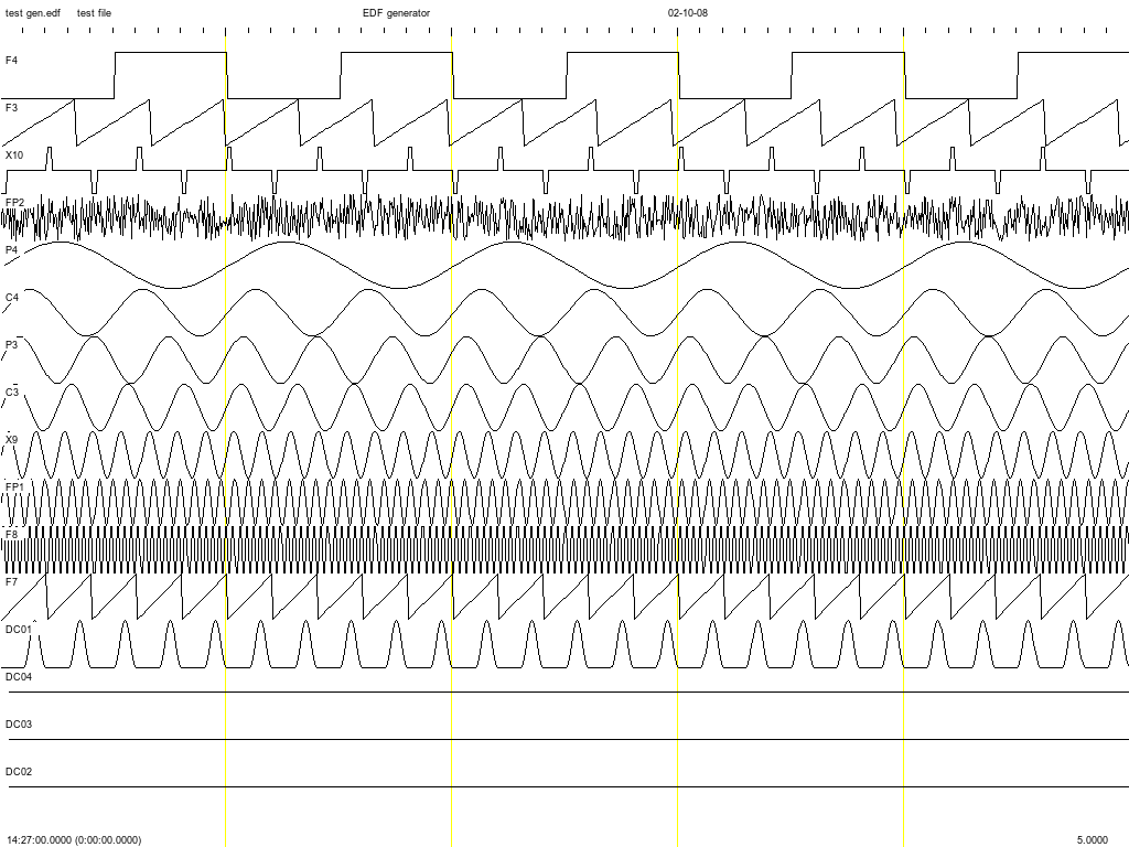
 signal label  waveform       physical range         f         sf
 --------------------------------------------------------------------
    1    F4     block          +800uV/-800uV          1Hz       200Hz
    2    F3     triangle       +800uV/-800uV          3Hz       100Hz
    3    X10    impulse        +0.8mV/-0.8mV          5Hz       200Hz
    4    FP2    noise          +3200uV/-3200uV        -Hz       200Hz
    5    P4     sine           +800uV/-800uV          1Hz        50Hz
    6    C4     sine           +800uV/-800uV          2Hz       100Hz
    7    P3     sine           +800uV/-800uV          3Hz       200Hz
    8    C3     sine           +800uV/-800uV          4Hz       200Hz
    9    X9     sine           +800uV/-800uV          8Hz       200Hz
   10    FP1    sine           +800uV/-800uV         16Hz       200Hz
   11    F8     sine           +800uV/-800uV         32Hz       200Hz
   12    F7     triangle       +4mV/-4mV              5Hz       200Hz
   13    DC01   sine square    +6V/-0V                5Hz       200Hz
   14    DC04   DC             +100%                  -Hz        25Hz
   15    DC03   DC             +60BPM                 -Hz        25Hz
   16    DC02   DC             +16384                 -Hz        25Hz
Thus, the uploaded data corresponds to the description of the test file, which confirms that the function is working correctly. edfread.
Let's build waveforms of the first 5 seconds of multi-channel recording to compare the resulting graphs with the test image.
t_max = 5.0     # time limit, with
nchan = size(record, 1) # number of channels

plt = plot(
    layout = (nchan, 1),
    size   = (1000, 200*nchan),
    margin = 20*Plots.px
)

for ch in 1:nchan
    # Channel sampling rate
    fs = hdr.samples[ch] / hdr.duration

    # Maximum number of samples per channel
    n_time = min(Int(round(t_max * fs)), hdr.samples[ch] * hdr.records)

    # Time and signal
    t = (0:n_time-1) ./ fs
    y = record[ch, 1:n_time]

    # Units of measurement
    units = hdr.physicalDims[ch]
    units = units == "" ? "-" : units

    plot!(
        plt[ch],
        t, y,
        label  = "$(hdr.labels[ch])",
        xlabel = "Time, from",
        ylabel = units,
        legend = :topright
    )
end

display(plt)
To test the function operation edfread using the extended EDF+ format, we will upload the file test_generator_2.edf.
hdr, record = edfread("$(@__DIR__)/test_generator_2.edf")
Similarly to the previous file, we extract and analyze the key parameters of the record.
println("Format version:         ", hdr.ver)
println("Patient ID:            ", strip(hdr.patientID))
println("Description of the record:        ", strip(hdr.recordID))
println("Start date/time:      ", hdr.startdate, " ", hdr.starttime)
println("Number of channels:     ", hdr.ns)
println("Number of entries:     ", hdr.records)
println("Total duration:     ", hdr.records * hdr.duration, " sec")
Let's create a table with the characteristics of each channel: its name, physical range of values, units of measurement, and sampling rate.
println("  No. | Channel | Range (min/max) | Unit | Frequency, Hz")
println("------------------------------------------------------------")

for ch in 1:hdr.ns-1
    label = hdr.labels[ch]

    # we take a row of the matrix and remove NaN (padding)
    row = record[ch, :]
    row = row[.!isnan.(row)]

    dataMin = round(minimum(row); digits = 2)
    dataMax = round(maximum(row); digits = 2)

    units = hdr.physicalDims[ch]
    units = units == "" ? "-" : units

    fs = round(hdr.samples[ch] / hdr.duration; digits = 2)

    println(
        lpad(ch, 2), " | ",
        rpad(label, 10), " | ",
        lpad(string(dataMin), 8), " / ",
        rpad(string(dataMax), 8), " | ",
        rpad(units, 6), " | ",
        fs
    )
end
To verify the correctness of reading and interpreting the data, we will compare the uploaded metadata with the reference information provided on the [EDF/BDF Test Files] page (https://teuniz.net/edf_bdf_testfiles /).
 signal label/waveform  amplitude    f       sf
---------------------------------------------------
   1    squarewave        100 uV    0.1Hz   200 Hz
   2    ramp              100 uV    1 Hz    200 Hz
   3    pulse             100 uV    1 Hz    200 Hz
   4    ECG               100 uV    1 Hz    200 Hz
   5    noise             100 uV    - Hz    200 Hz
   6    sine 1 Hz         100 uV    1 Hz    200 Hz
   7    sine 8 Hz         100 uV    8 Hz    200 Hz
   8    sine 8.5 Hz       100 uV    8.5Hz   200 Hz
   9    sine 15 Hz        100 uV   15 Hz    200 Hz
  10    sine 17 Hz        100 uV   17 Hz    200 Hz
  11    sine 50 Hz        100 uV   50 Hz    200 Hz
Thus, the uploaded data corresponds to the description of the test file, which confirms that the function is working correctly. edfread.
To check the correct functioning of the download and interpretation of EDF+ data, we will plot the graphs of the first 10 seconds of recording.
t_max = 10.0     # time limit, with
nchan = size(record, 1)-1

plt = plot(
    layout = (nchan, 1),
    size   = (1000, 200*nchan),
    margin = 30*Plots.px
)

for ch in 1:(nchan)
    # Channel sampling rate
    fs = hdr.samples[ch] / hdr.duration

    # Maximum number of samples per channel
    n_time = min(Int(round(t_max * fs)), hdr.samples[ch] * hdr.records)

    # Time and signal
    t = (0:n_time-1) ./ fs
    y = record[ch, 1:n_time]

    # Units of measurement
    units = hdr.physicalDims[ch]
    units = units == "" ? "-" : units

    plot!(
        plt[ch],
        t, y,
        label  = "$(hdr.labels[ch])",
        xlabel = "Time, from",
        ylabel = units,
        legend = :topright
    )
end

display(plt)
.png)
Conclusion
In this example, the principle of working with data in the EDF and EDF+ formats was considered. Using the example of test files (test_generator.edf and test_generator_2.edf), taken from [EDF/BDF Test Files](https://teuniz.net/edf_bdf_testfiles /).