Integrator Interface

The integrator interface gives one the ability to interactively step through the numerical solving of a differential equation. Through this interface, one can easily monitor results, modify the problem during a run, and dynamically continue solving as one sees fit.

Initialization and Stepping

To initialize an integrator, use the syntax:

integrator = init(prob, alg; kwargs...)

The keyword args which are accepted are the same as the solver options used by solve and the returned value is an integrator which satisfies typeof(integrator)<:DEIntegrator. One can manually choose to step via the step! command:

step!(integrator)

which will take one successful step. Additionally:

step!(integrator, dt, stop_at_tdt = false)

passing a dt will make the integrator continue to step until integrator.t+dt, and setting stop_at_tdt=true will add a tstop to force it to step to integrator.t+dt

To check whether the integration step was successful, you can call check_error(integrator) which returns one of the return codes.

This type also implements an iterator interface, so one can step n times (or to the last tstop) using the take iterator:

for i in take(integrator, n)
end

One can loop to the end by using solve!(integrator) or using the iterator interface:

for i in integrator
end

In addition, some helper iterators are provided to help monitor the solution. For example, the tuples iterator lets you view the values:

for (u, t) in tuples(integrator)
    @show u, t
end

and the intervals iterator lets you view the full interval:

for (uprev, tprev, u, t) in intervals(integrator)
    @show tprev, t
end

Additionally, you can make the iterator return specific time points via the TimeChoiceIterator:

ts = range(0, stop = 1, length = 11)
for (u, t) in TimeChoiceIterator(integrator, ts)
    @show u, t
end

Lastly, one can dynamically control the “endpoint”. The initialization simply makes prob.tspan[2] the last value of tstop, and many of the iterators are made to stop at the final tstop value. However, step! will always take a step, and one can dynamically add new values of tstops by modifying the variable in the options field: add_tstop!(integrator,new_t).

Finally, to solve to the last tstop, call solve!(integrator). Doing init and then solve! is equivalent to solve.

# CommonSolve.step! — Function

step!(integ::DEIntegrator [, dt [, stop_at_tdt]])

Perform one (successful) step on the integrator.

Alternative, if a dt is given, then step! the integrator until there is a temporal difference ≥ dt in integ.t. When true is passed to the optional third argument, the integrator advances exactly dt.

# SciMLBase.check_error — Function

check_error(integrator)

Check state of integrator and return one of the Return Codes

# SciMLBase.check_error! — Function

check_error!(integrator)

Same as check_error but also set solution’s return code (integrator.sol.retcode) and run postamble!.

Handling Integrators

The integrator<:DEIntegrator type holds all the information for the intermediate solution of the differential equation. Useful fields are:

t - time of the proposed step
u - value at the proposed step
p - user-provided data
opts - common solver options
alg - the algorithm associated with the solution
f - the function being solved
sol - the current state of the solution
tprev - the last timepoint
uprev - the value at the last timepoint
tdir - the sign for the direction of time

The function f is usually a wrapper of the function provided when creating the specific problem. For example, when solving an ODEProblem, f will be an ODEFunction. To access the right-hand side function provided by the user when creating the ODEProblem, please use SciMLBase.unwrapped_f(integrator.f.f).

The p is the (parameter) data which is provided by the user as a keyword arg in init. opts holds all the common solver options, and can be mutated to change the solver characteristics. For example, to modify the absolute tolerance for the future timesteps, one can do:

integrator.opts.abstol = 1e-9

The sol field holds the current solution. This current solution includes the interpolation function if available, and thus integrator.sol(t) lets one interpolate efficiently over the whole current solution. Additionally, a “current interval interpolation function” is provided on the integrator type via integrator(t,deriv::Type=Val{0};idxs=nothing,continuity=:left). This uses only the solver information from the interval [tprev,t] to compute the interpolation, and is allowed to extrapolate beyond that interval.

Note about mutating

Be cautious: one should not directly mutate the t and u fields of the integrator. Doing so will destroy the accuracy of the interpolator and can harm certain algorithms. Instead, if one wants to introduce discontinuous changes, one should use the callbacks. Modifications within a callback affect! surrounded by saves provides an error-free handling of the discontinuity.

As low-level alternative to the callbacks, one can use set_t!, set_u! and set_ut! to mutate integrator states. Note that certain integrators may not have efficient ways to modify u and t. In such case, set_*! are as inefficient as reinit!.

# SciMLBase.set_t! — Function

set_t!(integrator::DEIntegrator, t)

Set current time point of the integrator to t.

# SciMLBase.set_u! — Function

set_u!(integrator::DEIntegrator, u)
set_u!(integrator::DEIntegrator, sym, val)

Set current state of the integrator to u. Alternatively, set the state of variable sym to value val.

# SciMLBase.set_ut! — Function

set_ut!(integrator::DEIntegrator, u, t)

Set current state of the integrator to u and t

Integrator vs Solution

The integrator and the solution have very different actions because they have very different meanings. The typeof(sol) <: DESolution type is a type with history: it stores all the (requested) timepoints and interpolates/acts using the values closest in time. On the other hand, the typeof(integrator)<:DEIntegrator type is a local object. It only knows the times of the interval it currently spans, the current caches and values, and the current state of the solver (the current options, tolerances, etc.). These serve very different purposes:

The integrator's interpolation can extrapolate, both forward and backward in time. This is used to estimate events and is internally used for predictions.
The integrator is fully mutable upon iteration. This means that every time an iterator affect is used, it will take timesteps from the current time. This means that first(integrator)!=first(integrator) since the integrator will step once to evaluate the left and then step once more (not backtracking). This allows the iterator to keep dynamically stepping, though one should note that it may violate some immutability assumptions commonly made about iterators.

If one wants the solution object, then one can find it in integrator.sol.

Function Interface

In addition to the type interface, a function interface is provided which allows for safe modifications of the integrator type, and allows for uniform usage throughout the ecosystem (for packages/algorithms which implement the functions). The following functions make up the interface:

Saving Controls

# SciMLBase.savevalues! — Function

savevalues!(integrator::DEIntegrator,
  force_save=false) -> Tuple{Bool, Bool}

Try to save the state and time variables at the current time point, or the saveat point by using interpolation when appropriate. It returns a tuple that is (saved, savedexactly). If savevalues! saved value, then saved is true, and if savevalues! saved at the current time point, then savedexactly is true.

The saving priority/order is as follows:

save_on
- saveat
- force_save
- save_everystep

Caches

# SciMLBase.get_tmp_cache — Function

get_tmp_cache(i::DEIntegrator)

Returns a tuple of internal cache vectors which are safe to use as temporary arrays. This should be used for integrator interface and callbacks which need arrays to write into in order to be non-allocating. The length of the tuple is dependent on the method.

# SciMLBase.full_cache — Function

full_cache(i::DEIntegrator)

Returns an iterator over the cache arrays of the method. This can be used to change internal values as needed.

Stepping Controls

# SciMLBase.u_modified! — Function

u_modified!(i::DEIntegrator,bool)

Sets bool which states whether a change to u occurred, allowing the solver to handle the discontinuity. By default, this is assumed to be true if a callback is used. This will result in the re-calculation of the derivative at t+dt, which is not necessary if the algorithm is FSAL and u does not experience a discontinuous change at the end of the interval. Thus, if u is unmodified in a callback, a single call to the derivative calculation can be eliminated by u_modified!(integrator,false).

# SciMLBase.get_proposed_dt — Function

get_proposed_dt(i::DEIntegrator)

Gets the proposed dt for the next timestep.

# SciMLBase.set_proposed_dt! — Function

set_proposed_dt(i::DEIntegrator,dt)
set_proposed_dt(i::DEIntegrator,i2::DEIntegrator)

Sets the proposed dt for the next timestep. If the second argument isa DEIntegrator, then it sets the timestepping of the first argument to match that of the second one. Note that due to PI control and step acceleration, this is more than matching the factors in most cases.

# SciMLBase.terminate! — Function

terminate!(i::DEIntegrator[, retcode = :Terminated])

Terminates the integrator by emptying tstops. This can be used in events and callbacks to immediately end the solution process. Optionally, retcode may be specified (see: Return Codes (RetCodes)).

# SciMLBase.change_t_via_interpolation! — Function

change_t_via_interpolation!(integrator::DEIntegrator,t,modify_save_endpoint=Val{false})

Modifies the current t and changes all of the corresponding values using the local interpolation. If the current solution has already been saved, one can provide the optional value modify_save_endpoint to also modify the endpoint of sol in the same manner.

# SciMLBase.add_tstop! — Function

add_tstop!(i::DEIntegrator,t)

Adds a tstop at time t.

# SciMLBase.has_tstop — Function

has_tstop(i::DEIntegrator)

Checks if integrator has any stopping times defined.

# SciMLBase.first_tstop — Function

first_tstop(i::DEIntegrator)

Gets the first stopping time of the integrator.

# SciMLBase.pop_tstop! — Function

pop_tstop!(i::DEIntegrator)

Pops the last stopping time from the integrator.

# SciMLBase.add_saveat! — Function

add_saveat!(i::DEIntegrator,t)

Adds a saveat time point at t.

Resizing

# Base.resize! — Function

resize!(integrator::DEIntegrator,k::Int)

Resizes the DE to a size k. This chops off the end of the array, or adds blank values at the end, depending on whether k > length(integrator.u).

# Base.deleteat! — Function

deleteat!(integrator::DEIntegrator,idxs)

Shrinks the ODE by deleting the idxs components.

# SciMLBase.addat! — Function

addat!(integrator::DEIntegrator,idxs,val)

Grows the ODE by adding the idxs components. Must be contiguous indices.

# SciMLBase.resize_non_user_cache! — Function

resize_non_user_cache!(integrator::DEIntegrator,k::Int)

Resizes the non-user facing caches to be compatible with a DE of size k. This includes resizing Jacobian caches.

In many cases, resize! simply resizes full_cache variables and then calls this function. This finer control is required for some AbstractArray operations.

# SciMLBase.deleteat_non_user_cache! — Function

deleteat_non_user_cache!(integrator::DEIntegrator,idxs)

deleteat!s the non-user facing caches at indices idxs. This includes resizing Jacobian caches.

In many cases, deleteat! simply deleteat!s full_cache variables and then calls this function. This finer control is required for some AbstractArray operations.

# SciMLBase.addat_non_user_cache! — Function

addat_non_user_cache!(i::DEIntegrator,idxs)

addat!s the non-user facing caches at indices idxs. This includes resizing Jacobian caches.

In many cases, addat! simply addat!s full_cache variables and then calls this function. This finer control is required for some AbstractArray operations.

Reinitialization

# SciMLBase.reinit! — Function

reinit!(integrator::DEIntegrator,args...; kwargs...)

The reinit function lets you restart the integration at a new value.

Arguments

u0: Value of u to start at. Default value is integrator.sol.prob.u0

Keyword Arguments

t0: Starting timepoint. Default value is integrator.sol.prob.tspan[1]
tf: Ending timepoint. Default value is integrator.sol.prob.tspan[2]
erase_sol=true: Whether to start with no other values in the solution, or keep the previous solution.
tstops, d_discontinuities, & saveat: Cache where these are stored. Default is the original cache.
reset_dt: Set whether to reset the current value of dt using the automatic dt determination algorithm. Default is (integrator.dtcache == zero(integrator.dt)) && integrator.opts.adaptive
reinit_callbacks: Set whether to run the callback initializations again (and initialize_save is for that). Default is true.
reinit_cache: Set whether to re-run the cache initialization function (i.e. resetting FSAL, not allocating vectors) which should usually be true for correctness. Default is true.

Additionally, once can access auto_dt_reset! which will run the auto dt initialization algorithm.

# SciMLBase.auto_dt_reset! — Function

auto_dt_reset!(integrator::DEIntegrator)

Run the auto dt initialization algorithm.

Misc

# SciMLBase.get_du — Function

get_du(i::DEIntegrator)

Returns the derivative at t.

# SciMLBase.get_du! — Function

get_du!(out,i::DEIntegrator)

Write the current derivative at t into out.

Note that not all these functions will be implemented for every algorithm. Some have hard limitations. For example, Sundials.jl cannot resize problems. When a function is not limited, an error will be thrown.

Additional Options

The following options can additionally be specified in init (or be mutated in the opts) for further control of the integrator:

advance_to_tstop: This makes step! continue to the next value in tstop.
stop_at_next_tstop: This forces the iterators to stop at the next value of tstop.

For example, if one wants to iterate but only stop at specific values, one can choose:

integrator = init(prob, Tsit5(); dt = 1 // 2^(4), tstops = [0.5], advance_to_tstop = true)
for (u, t) in tuples(integrator)
    @test t ∈ [0.5, 1.0]
end

which will only enter the loop body at the values in tstops (here, prob.tspan[2]==1.0 and thus there are two values of tstops which are hit). Additionally, one can solve! only to 0.5 via:

integrator = init(prob, Tsit5(); dt = 1 // 2^(4), tstops = [0.5])
integrator.opts.stop_at_next_tstop = true
solve!(integrator)

Plot Recipe

Like the DESolution type, a plot recipe is provided for the DEIntegrator type. Since the DEIntegrator type is a local state type on the current interval, plot(integrator) returns the solution on the current interval. The same options for the plot recipe are provided as for sol, meaning one can choose variables via the idxs keyword argument, or change the plotdensity / turn on/off denseplot.

Additionally, since the integrator is an iterator, this can be used in the Plots.jl animate command to iteratively build an animation of the solution while solving the differential equation.

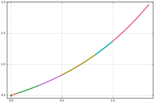
For an example of manually chaining together the iterator interface and plotting, one should try the following:

using DifferentialEquations, DiffEqProblemLibrary, Plots

# Linear ODE which starts at 0.5 and solves from t=0.0 to t=1.0
prob = ODEProblem((u, p, t) -> 1.01u, 0.5, (0.0, 1.0))

using Plots
integrator = init(prob, Tsit5(); dt = 1 // 2^(4), tstops = [0.5])
pyplot(show = true)
plot(integrator)
for i in integrator
    display(plot!(integrator, idxs = (0, 1), legend = false))
end
step!(integrator);
plot!(integrator, idxs = (0, 1), legend = false);
savefig("iteratorplot.png")