Overarching tutorial for DynamicalSystems.jl
This page serves as a short, but to-the-point, introduction to the DynamicalSystems.jl library. It outlines the core components, and how they establish an interface that is used by the rest of the library. It also provides a couple of usage examples to connect the various packages of the library together.
Going through this tutorial should take you about 20 minutes.
Installation
To install DynamicalSystems.jl, simply do:
using Pkg; Pkg.add("DynamicalSystems")As discussed in the contents page, this installs several packages for the Julia language, that are all exported under a common name. To use them, simply do:
using DynamicalSystemsin your Julia session.
Core components
The individual packages that compose DynamicalSystems interact flawlessly with each other because of the following two components:
-
The
StateSpaceSet, which represents numerical data. They can be observed or measured from experiments, sampled trajectories of dynamical systems, or just unordered sets in a state space. AStateSpaceSetis a container of equally-sized points, representing multivariate timeseries or multivariate datasets. Timeseries, which are univariate sets, are represented by theAbstractVector{<:Real}Julia base type. -
The
DynamicalSystem, which is the abstract representation of a dynamical system with a known dynamic evolution rule.DynamicalSystemdefines an extendable interface, but typically one uses concrete implementations such asDeterministicIteratedMaporCoupledODEs.
Making dynamical systems
In the majority of cases, to make a dynamical system one needs three things:
-
The dynamic rule
f: A Julia function that provides the instructions of how to evolve the dynamical system in time. -
The state
u: An array-like container that contains the variables of the dynamical system and also defines the starting state of the system. -
The parameters
p: An arbitrary container that parameterizesf.
For most concrete implementations of DynamicalSystem there are two ways of defining f, u. The distinction is done on whether f is defined as an in-place (iip) function or out-of-place (oop) function.
-
oop :
fmust be in the formf(u, p, t) -> outwhich means that given a stateu::SVector{<:Real}and some parameter containerpit returns the output offas anSVector{<:Real}(static vector). -
iip :
fmust be in the formf!(out, u, p, t)which means that given a stateu::AbstractArray{<:Real}and some parameter containerp, it writes in-place the output offinout::AbstractArray{<:Real}. The function must returnnothingas a final statement.
t stands for current time in both cases. iip is suggested for systems with high dimension and oop for small. The break-even point is between 10 to 100 dimensions but should be benchmarked on a case-by-case basis as it depends on the complexity of f.
Example: Henon map
Let’s make the Henon map, defined as
with parameters .
First, we define the dynamic rule as a standard Julia function. Since the dynamical system is only two-dimensional, we should use the out-of-place form that returns an SVector with the next state:
using DynamicalSystems

function henon_rule(u, p, n) # here `n` is "time", but we don't use it.
    x, y = u # system state
    a, b = p # system parameters
    xn = 1.0 - a*x^2 + y
    yn = b*x
    return SVector(xn, yn)
end
henon_rule (generic function with 1 method)Then, we define initial state and parameters
u0 = [0.2, 0.3]
p0 = [1.4, 0.3]
2-element Vector{Float64}:
1.4
0.3Lastly, we give these three to the DeterministicIteratedMap:
henon = DeterministicIteratedMap(henon_rule, u0, p0)2-dimensional DeterministicIteratedMap
deterministic: true
discrete time: true
in-place: false
dynamic rule: henon_rule
parameters: [1.4, 0.3]
time: 0
state: [0.2, 0.3]henon is a DynamicalSystem, one of the two core structures of the library. They can evolved interactively, and queried, using the interface defined by DynamicalSystem. The simplest thing you can do with a DynamicalSystem is to get its trajectory:
total_time = 10_000
X, t = trajectory(henon, total_time)
(2-dimensional StateSpaceSet{Float64} with 10001 points, 0:1:10000)X2-dimensional StateSpaceSet{Float64} with 10001 points
0.2 0.3
1.244 0.06
-1.10655 0.3732
-0.341035 -0.331965
0.505208 -0.102311
0.540361 0.151562
0.742777 0.162108
0.389703 0.222833
1.01022 0.116911
-0.311842 0.303065
⋮
-0.582534 0.328346
0.853262 -0.17476
-0.194038 0.255978
1.20327 -0.0582113
-1.08521 0.36098
-0.287758 -0.325562
0.558512 -0.0863275
0.476963 0.167554
0.849062 0.143089X is a StateSpaceSet, the second of the core structures of the library. We’ll see below how, and where, to use a StateSpaceset, but for now let’s just do a scatter plot
using CairoMakie
scatter(X[:, 1], X[:, 2])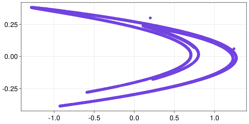
Example: Lorenz96
Let’s also make another dynamical system, the Lorenz96 model:
for and .
Here, instead of a discrete time map we have coupled ordinary differential equations. However, creating the dynamical system works out just like above, but using CoupledODEs instead of DeterministicIteratedMap.
First, we make the dynamic rule function. Since this dynamical system can be arbitrarily high-dimensional, we prefer to use the in-place form for f, overwriting in place the rate of change in a pre-allocated container. It is customary to append the name of functions that modify their arguments in-place with a bang (!).
function lorenz96_rule!(du, u, p, t)
    F = p[1]; N = length(u)
    # 3 edge cases
    du[1] = (u[2] - u[N - 1]) * u[N] - u[1] + F
    du[2] = (u[3] - u[N]) * u[1] - u[2] + F
    du[N] = (u[1] - u[N - 2]) * u[N - 1] - u[N] + F
    # then the general case
    for n in 3:(N - 1)
        du[n] = (u[n + 1] - u[n - 2]) * u[n - 1] - u[n] + F
    end
    return nothing # always `return nothing` for in-place form!
end
lorenz96_rule! (generic function with 1 method)then, like before, we define an initial state and parameters, and initialize the system
N = 6
u0 = range(0.1, 1; length = N)
p0 = [8.0]
lorenz96 = CoupledODEs(lorenz96_rule!, u0, p0)
6-dimensional CoupledODEs
deterministic: true
discrete time: false
in-place: true
dynamic rule: lorenz96_rule!
ODE solver: Tsit5
ODE kwargs: (abstol = 1.0e-6, reltol = 1.0e-6)
parameters: [8.0]
time: 0.0
state: [0.1, 0.28, 0.46, 0.64, 0.82, 1.0]and, again like before, we may obtain a trajectory the same way
total_time = 12.5
sampling_time = 0.02
Y, t = trajectory(lorenz96, total_time; Ttr = 2.2, Δt = sampling_time)
Y
6-dimensional StateSpaceSet{Float64} with 626 points
3.15368 -4.40493 0.0311581 0.486735 1.89895 4.15167
2.71382 -4.39303 0.395019 0.66327 2.0652 4.32045
2.25088 -4.33682 0.693967 0.879701 2.2412 4.46619
1.7707 -4.24045 0.924523 1.12771 2.42882 4.58259
1.27983 -4.1073 1.08656 1.39809 2.62943 4.66318
0.785433 -3.94005 1.18319 1.6815 2.84384 4.70147
0.295361 -3.74095 1.2205 1.96908 3.07224 4.69114
-0.181932 -3.51222 1.20719 2.25296 3.3139 4.62628
-0.637491 -3.25665 1.154 2.5267 3.56698 4.50178
-1.06206 -2.9781 1.07303 2.7856 3.82827 4.31366
⋮ ⋮
3.17245 2.3759 3.01796 7.27415 7.26007 -0.116002
3.29671 2.71146 3.32758 7.5693 6.75971 -0.537853
3.44096 3.09855 3.66908 7.82351 6.13876 -0.922775
3.58387 3.53999 4.04452 8.01418 5.39898 -1.25074
3.70359 4.03513 4.45448 8.1137 4.55005 -1.5042
3.78135 4.57879 4.89677 8.09013 3.61125 -1.66943
3.80523 5.16112 5.36441 7.90891 2.61262 -1.73822
3.77305 5.7684 5.84318 7.53627 1.59529 -1.71018
3.6934 6.38507 6.30923 6.94454 0.61023 -1.59518We can’t scatterplot something 6-dimensional but we can visualize all timeseries
fig = Figure()
ax = Axis(fig[1, 1]; xlabel = "time", ylabel = "variable")
for var in columns(Y)
    lines!(ax, t, var)
end
fig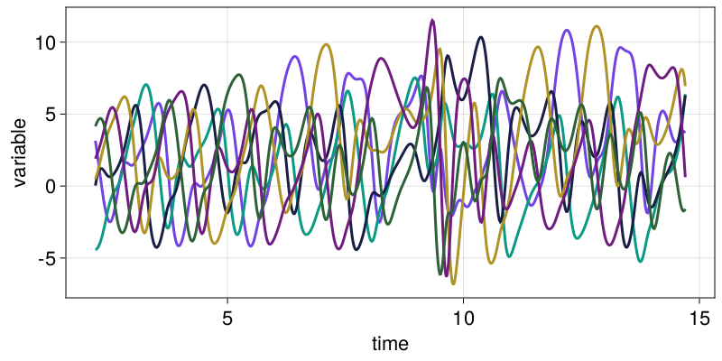
ODE solving
Continuous time dynamical systems are evolved through DifferentialEquations.jl. When initializing a CoupledODEs you can tune the solver properties to your heart’s content using any of the ODE solvers and any of the common solver options. For example:
using OrdinaryDiffEq # accessing the ODE solvers
diffeq = (alg = Vern9(), abstol = 1e-9, reltol = 1e-9)
lorenz96_vern = ContinuousDynamicalSystem(lorenz96_rule!, u0, p0; diffeq)
6-dimensional CoupledODEs
deterministic: true
discrete time: false
in-place: true
dynamic rule: lorenz96_rule!
ODE solver: Vern9
ODE kwargs: (abstol = 1.0e-9, reltol = 1.0e-9)
parameters: [8.0]
time: 0.0
state: [0.1, 0.28, 0.46, 0.64, 0.82, 1.0]Y, t = trajectory(lorenz96_vern, total_time; Ttr = 2.2, Δt = sampling_time)
Y[end]6-element SVector{6, Float64} with indices SOneTo(6):
3.8390248122550252
6.1557095311542325
6.080625689025621
7.278588308988913
1.2582152212831657
-1.5297062916833186Using dynamical systems
You may use the DynamicalSystem interface to develop algorithms that utilize dynamical systems with a known evolution rule. The two main packages of the library that do this are ChaosTools and Attractors. For example, you may want to compute the Lyapunov spectrum of the Lorenz96 system from above. This is as easy as calling the lyapunovspectrum function with lorenz96
steps = 10_000
lyapunovspectrum(lorenz96, steps)
6-element Vector{Float64}:
0.9578297436475178
0.0007190960151481466
-0.15749134695138844
-0.7575338861926539
-1.4036253850302072
-4.639894729260599As expected, there is at least one positive Lyapunov exponent (before the system is chaotic) and at least one zero Lyapunov exponent, because the system is continuous time.
Alternatively, you may want to estimate the basins of attraction of a multistable dynamical system. The Henon map is "multistable" in the sense that some initial conditions diverge to infinity, and some others converge to a chaotic attractor. Computing these basins of attraction is simple with Attractors, and would work as follows:
# define a state space grid to compute the basins on:
xg = yg = range(-2, 2; length = 201)
# find attractors using recurrences in state space:
mapper = AttractorsViaRecurrences(henon, (xg, yg); sparse = false)
# compute the full basins of attraction:
basins, attractors = basins_of_attraction(mapper; show_progress = false)
(Int32[-1 -1 … -1 -1; -1 -1 … -1 -1; … ; -1 -1 … -1 -1; -1 -1 … -1 -1], Dict{Int32, StateSpaceSet{2, Float64}}(1 => 2-dimensional StateSpaceSet{Float64} with 511 points))fig, ax = heatmap(xg, yg, basins)
x, y = columns(X) # attractor of Henon map
scatter!(ax, x, y; color = "black")
fig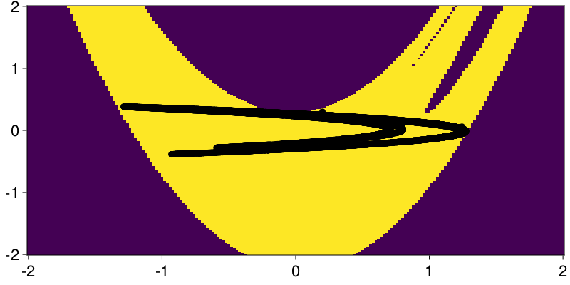
You could also be using a DynamicalSystem instance directly to build your own algorithm if it isn’t already implemented (and then later contribute it so it is implemented ;) ). A dynamical system can be evolved forwards in time using step!:
henon2-dimensional DeterministicIteratedMap
deterministic: true
discrete time: true
in-place: false
dynamic rule: henon_rule
parameters: [1.4, 0.3]
time: 5
state: [-1.5266434026801804e8, -3132.7519146699206]Notice how the time is not 0, because henon has already been stepped when we called the function basins_of_attraction with it. We can step it more:
step!(henon)2-dimensional DeterministicIteratedMap
deterministic: true
discrete time: true
in-place: false
dynamic rule: henon_rule
parameters: [1.4, 0.3]
time: 6
state: [-3.262896110526e16, -4.579930208040541e7]step!(henon, 2)2-dimensional DeterministicIteratedMap
deterministic: true
discrete time: true
in-place: false
dynamic rule: henon_rule
parameters: [1.4, 0.3]
time: 8
state: [-3.110262842032839e66, -4.4715262317959936e32]For more information on how to directly use DynamicalSystem instances, see the documentation of DynamicalSystemsBase.
State space sets
Let’s recall that the output of the trajectory function is a StateSpaceSet:
X2-dimensional StateSpaceSet{Float64} with 10001 points
0.2 0.3
1.244 0.06
-1.10655 0.3732
-0.341035 -0.331965
0.505208 -0.102311
0.540361 0.151562
0.742777 0.162108
0.389703 0.222833
1.01022 0.116911
-0.311842 0.303065
⋮
-0.582534 0.328346
0.853262 -0.17476
-0.194038 0.255978
1.20327 -0.0582113
-1.08521 0.36098
-0.287758 -0.325562
0.558512 -0.0863275
0.476963 0.167554
0.849062 0.143089It is printed like a matrix where each column is the timeseries of each dynamic variable. In reality, it is a vector of statically sized vectors (for performance reasons). When indexed with 1 index, it behaves like a vector of vectors
X[1]2-element SVector{2, Float64} with indices SOneTo(2):
0.2
0.3X[2:5]2-dimensional StateSpaceSet{Float64} with 4 points
1.244 0.06
-1.10655 0.3732
-0.341035 -0.331965
0.505208 -0.102311When indexed with two indices, it behaves like a matrix
X[2:5, 2]4-element Vector{Float64}:
0.06
0.3732
-0.3319651199999999
-0.10231059085086688When iterated, it iterates over the contained points
for (i, point) in enumerate(X)
    @show point
    i > 5 && break
end
point = [0.2, 0.3]
point = [1.244, 0.06]
point = [-1.1065503999999997, 0.3732]
point = [-0.34103530283622296, -0.3319651199999999]
point = [0.5052077711071681, -0.10231059085086688]
point = [0.5403605603672313, 0.1515623313321504]map(point -> point[1] + point[2], X)10001-element Vector{Float64}:
0.5
1.304
-0.7333503999999997
-0.6730004228362229
0.40289718025630117
0.6919228916993818
0.9048851501617762
0.6125365596336813
1.1271278272148746
-0.008777065619615998
⋮
-0.2541879392427324
0.678501271515278
0.061940665344374896
1.145056192451011
-0.7242249528790483
-0.6133198017049188
0.47218423998951875
0.6445165778497133
0.9921511619004666The columns of the set are obtained with the convenience columns function
x, y = columns(X)
summary.((x, y))
("10001-element Vector{Float64}", "10001-element Vector{Float64}")Using state space sets
Several packages of the library deal with StateSpaceSets.
You could use ComplexityMeasures to obtain the entropy, or other complexity measures, of a given set. Below, we obtain the entropy of the natural density of the chaotic attractor by partitioning into a histogram of approximately 50 bins per dimension:
prob_est = ValueHistogram(50)
entropy(prob_est, X)7.825799208736613Alternatively, you could use FractalDimensions to get the fractal dimensions of the chaotic attractor of the henon map using the Grassberger-Procaccia algorithm:
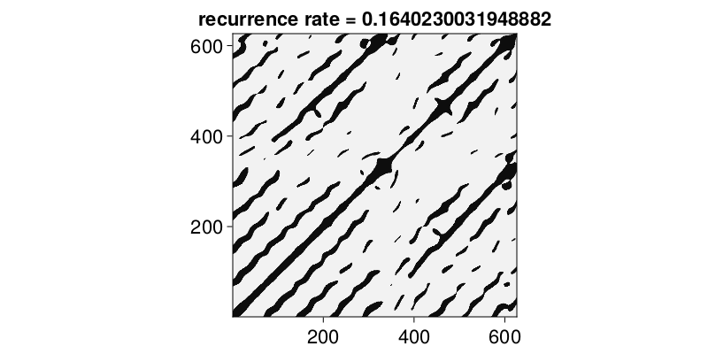
grassberger_proccacia_dim(X)1.2232922815092426Or, you could obtain a recurrence matrix of a state space set with RecurrenceAnalysis
R = RecurrenceMatrix(Y, 8.0)
Rg = grayscale(R)
rr = recurrencerate(R)
heatmap(Rg; colormap = :grays,
    axis = (title = "recurrence rate = $(rr)", aspect = 1,)
)
More nonlinear timeseries analysis
A trajectory of a known dynamical system is one way to obtain a StateSpaceSet. However, another common way is via a delay coordinates embedding of a measured/observed timeseries. For example, we could use optimal_separated_de from DelayEmbeddings to create an optimized delay coordinates embedding of a timeseries
w = Y[:, 1] # first variable of Lorenz96
𝒟, τ, e = optimal_separated_de(w)
𝒟
5-dimensional StateSpaceSet{Float64} with 558 points
3.15369 -2.40036 1.60497 2.90499 5.72572
2.71384 -2.24811 1.55832 3.04987 5.6022
2.2509 -2.02902 1.50499 3.20633 5.38629
1.77073 -1.75077 1.45921 3.37699 5.07029
1.27986 -1.42354 1.43338 3.56316 4.65003
0.785468 -1.05974 1.43672 3.76473 4.12617
0.295399 -0.673567 1.47423 3.98019 3.50532
-0.181891 -0.280351 1.54635 4.20677 2.80048
-0.637447 0.104361 1.64932 4.44054 2.03084
-1.06201 0.465767 1.77622 4.67654 1.22067
⋮
7.42111 9.27879 -1.23936 5.15945 3.25618
7.94615 9.22663 -1.64222 5.24344 3.34749
8.40503 9.13776 -1.81947 5.26339 3.46932
8.78703 8.99491 -1.77254 5.22631 3.60343
9.08701 8.77963 -1.51823 5.13887 3.72926
9.30562 8.47357 -1.08603 5.00759 3.82705
9.4488 8.06029 -0.514333 4.83928 3.88137
9.52679 7.52731 0.153637 4.6414 3.88458
9.55278 6.86845 0.873855 4.42248 3.83902and compare
fig = Figure()
axs = [Axis3(fig[1, i]) for i in 1:2]
for (S, ax) in zip((Y, 𝒟), axs)
    lines!(ax, S[:, 1], S[:, 2], S[:, 3])
end
fig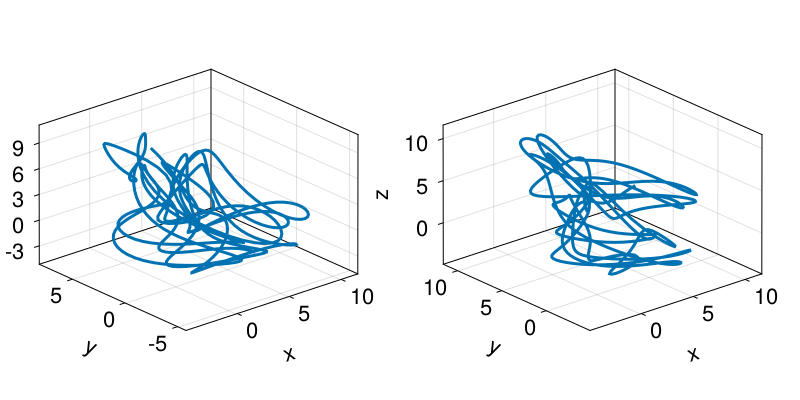
Since 𝒟 is just another state space set, we could be using any of the above analysis pipelines on it just as easily.
The last package to mention here is TimeseriesSurrogates, which ties with all other observed/measured data analysis by providing a framework for confidence/hypothesis testing. For example, if we had a measured timeseries but we were not sure whether it represents a deterministic system with structure in the state space, or mostly noise, we could do a surrogate test. For this, we use surrogenerator and RandomFourier from TimeseriesSurrogates, and the generalized_dim from FractalDimensions (because it performs better in noisy sets)
x = X[:, 1] # Henon map timeseries
# contaminate with noise
using Random: Xoshiro
rng = Xoshiro(1234)
x .+= randn(rng, length(x))/100
# compute noise-contaminated fractal dim.
Δ_orig = generalized_dim(embed(x, 2, 1))1.3801073957979793And we do the surrogate test
surrogate_method = RandomFourier()
sgen = surrogenerator(x, surrogate_method, rng)

Δ_surr = map(1:1000) do i
    s = sgen()
    generalized_dim(embed(s, 2, 1))
end
1000-element Vector{Float64}:
1.8297218640747606
1.8449246422083758
1.827998413768852
1.8301078704767055
1.810704251592814
1.8324978359365702
1.8300954188512213
1.8416570396197014
1.8575804541517287
1.821435647618282
⋮
1.8768262063118628
1.8287938131103985
1.8435474417451545
1.8129026565561648
1.8551700924676993
1.8283378225272842
1.8211346475312316
1.8369834750866052
1.8368699339310082and visualize the test result
fig, ax = hist(Δ_surr)
vlines!(ax, Δ_orig)
fig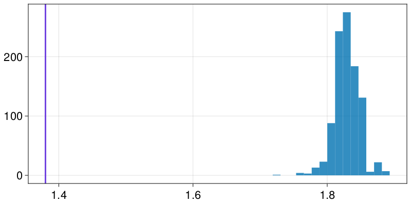
since the real value is outside the distribution we have confidence the data are not pure noise.
Core components reference
#
StateSpaceSets.StateSpaceSet — Type
StateSpaceSet{D, T} <: AbstractStateSpaceSet{D,T}A dedicated interface for sets in a state space. It is an ordered container of equally-sized points of length D. Each point is represented by SVector{D, T}. The data are a standard Julia Vector{SVector}, and can be obtained with vec(ssset::StateSpaceSet). Typically the order of points in the set is the time direction, but it doesn’t have to be.
When indexed with 1 index, StateSpaceSet is like a vector of points. When indexed with 2 indices it behaves like a matrix that has each of the columns be the timeseries of each of the variables. When iterated over, it iterates over its contained points. See description of indexing below for more.
StateSpaceSet also supports almost all sensible vector operations like append!, push!, hcat, eachrow, among others.
Description of indexing
In the following let i, j be integers, typeof(X) <: AbstractStateSpaceSet and v1, v2 be <: AbstractVector{Int} (v1, v2 could also be ranges, and for performance benefits make v2 an SVector{Int}).
-
X[i] == X[i, :]gives theith point (returns anSVector) -
X[v1] == X[v1, :], returns aStateSpaceSetwith the points in those indices. -
X[:, j]gives thejth variable timeseries (or collection), asVector -
X[v1, v2], X[:, v2]returns aStateSpaceSetwith the appropriate entries (first indices being "time"/point index, while second being variables) -
X[i, j]value of thejth variable, at theith timepoint
Use Matrix(ssset) or StateSpaceSet(matrix) to convert. It is assumed that each column of the matrix is one variable. If you have various timeseries vectors x, y, z, ... pass them like StateSpaceSet(x, y, z, ...). You can use columns(dataset) to obtain the reverse, i.e. all columns of the dataset in a tuple.
#
DynamicalSystemsBase.DynamicalSystem — Type
DynamicalSystemDynamicalSystem is an abstract supertype encompassing all concrete implementations of what counts as a "dynamical system" in the DynamicalSystems.jl library.
All concrete implementations of DynamicalSystem can be iteratively evolved in time via the step! function. Hence, most library functions that evolve the system will mutate its current state and/or parameters. See the documentation online for implications this has on for parallelization.
DynamicalSystem is further separated into two abstract types: ContinuousTimeDynamicalSystem, DiscreteTimeDynamicalSystem. The simplest and most common concrete implementations of a DynamicalSystem are DeterministicIteratedMap or CoupledODEs.
Description
|
The documentation of |
A ds::DynamicalSystem representes a flow Φ in a state space. It mainly encapsulates three things:
-
A state, typically referred to as
u, with initial valueu0. The space thatuoccupies is the state space ofdsand the length ofuis the dimension ofds(and of the state space). -
A dynamic rule, typically referred to as
f, that dictates how the state evolves/changes with time when calling thestep!function.fis a standard Julia function, see below. -
A parameter container
pthat parameterizesf.pcan be anything, but in general it is recommended to be a type-stable mutable container.
In sort, any set of quantities that change in time can be considered a dynamical system, however the concrete subtypes of DynamicalSystem are much more specific in their scope. Concrete subtypes typically also contain more information than the above 3 items.
In this scope dynamical systems have a known dynamic rule f defined as a standard Julia function. Observed or measured data from a dynamical system are represented using StateSpaceSet and are finite. Such data are obtained from the trajectory function or from an experimental measurement of a dynamical system with an unknown dynamic rule.
Construction instructions on f and u
Most of the concrete implementations of DynamicalSystem, with the exception of ArbitrarySteppable, have two ways of implementing the dynamic rule f, and as a consequence the type of the state u. The distinction is done on whether f is defined as an in-place (iip) function or out-of-place (oop) function.
-
oop :
fmust be in the formf(u, p, t) -> outwhich means that given a stateu::SVector{<:Real}and some parameter containerpit returns the output offas anSVector{<:Real}(static vector). -
iip :
fmust be in the formf!(out, u, p, t)which means that given a stateu::AbstractArray{<:Real}and some parameter containerp, it writes in-place the output offinout::AbstractArray{<:Real}. The function must returnnothingas a final statement.
t stands for current time in both cases. iip is suggested for systems with high dimension and oop for small. The break-even point is between 10 to 100 dimensions but should be benchmarked on a case-by-case basis as it depends on the complexity of f.
|
Whether the dynamical system is autonomous ( |
API
The API that the interface of DynamicalSystem employs is the functions listed below. Once a concrete instance of a subtype of DynamicalSystem is obtained, it can quieried or altered with the following functions.
The main use of a concrete dynamical system instance is to provide it to downstream functions such as lyapunovspectrum from ChaosTools.jl or basins_of_attraction from Attractors.jl. A typical user will likely not utilize directly the following API, unless when developing new algorithm implementations that use dynamical systems.
API - information
-
ds(t)withdsan instance ofDynamicalSystem: return the state ofdsat timet. For continuous time systems this interpolates and extrapolates, while for discrete time systems it only works iftis the current time.
API - alter status
Dynamical system implementations
#
DynamicalSystemsBase.DeterministicIteratedMap — Type
DeterministicIteratedMap <: DynamicalSystem
DeterministicIteratedMap(f, u0, p = nothing; t0 = 0)
A deterministic discrete time dynamical system defined by an iterated map as follows:
An alias for DeterministicIteratedMap is DiscreteDynamicalSystem.
Optionally configure the parameter container p and initial time t0.
For construction instructions regarding f, u0 see DynamicalSystem.
#
DynamicalSystemsBase.CoupledODEs — Type
CoupledODEs <: ContinuousTimeDynamicalSystem
CoupledODEs(f, u0 [, p]; diffeq, t0 = 0.0)
A deterministic continuous time dynamical system defined by a set of coupled ordinary differential equations as follows:
An alias for CoupledODE is ContinuousDynamicalSystem.
Optionally provide the parameter container p and initial time as keyword t0.
For construction instructions regarding f, u0 see DynamicalSystem.
DifferentialEquations.jl keyword arguments and interfacing
The ODEs are evolved via the solvers of DifferentialEquations.jl. When initializing a CoupledODEs, you can specify the solver that will integrate f in time, along with any other integration options, using the diffeq keyword. For example you could use diffeq = (abstol = 1e-9, reltol = 1e-9). If you want to specify a solver, do so by using the keyword alg, e.g.: diffeq = (alg = Tsit5(), reltol = 1e-6). This requires you to have been first using OrdinaryDiffEq to access the solvers. The default diffeq is:
(alg = Tsit5(; stagelimiter! = triviallimiter!, steplimiter! = triviallimiter!, thread = static(false),), abstol = 1.0e-6, reltol = 1.0e-6)
diffeq keywords can also include callback for event handling, however the majority of downstream functions in DynamicalSystems.jl assume that f is differentiable.
The convenience constructor CoupledODEs(prob::ODEProblem, diffeq) and CoupledODEs(ds::CoupledODEs, diffeq) are also available.
Dev note: CoupledODEs is a light wrapper of ODEIntegrator from DifferentialEquations.jl. The integrator is available as the field integ, and the ODEProblem is integ.sol.prob. The convenience syntax ODEProblem(ds::CoupledODEs, tspan = (t0, Inf)) is available.
#
DynamicalSystemsBase.StroboscopicMap — Type
StroboscopicMap <: DiscreteTimeDynamicalSystem
StroboscopicMap(ds::CoupledODEs, period::Real) → smap
StroboscopicMap(period::Real, f, u0, p = nothing; kwargs...)
A discrete time dynamical system that produces iterations of a time-dependent (non-autonomous) CoupledODEs system exactly over a given period. The second signature first creates a CoupledODEs and then calls the first.
StroboscopicMap follows the DynamicalSystem interface. In addition, the function set_period!(smap, period) is provided, that sets the period of the system to a new value (as if it was a parameter). As this system is in discrete time, current_time and initial_time are integers. The initial time is always 0, because current_time counts elapsed periods. Call these functions on the parent of StroboscopicMap to obtain the corresponding continuous time. In contrast, reinit! expects t0 in continuous time.
The convenience constructor
StroboscopicMap(T::Real, f, u0, p = nothing; diffeq, t0 = 0) → smapis also provided.
See also PoincareMap.
#
DynamicalSystemsBase.PoincareMap — Type
PoincareMap <: DiscreteTimeDynamicalSystem
PoincareMap(ds::CoupledODEs, plane; kwargs...) → pmap
A discrete time dynamical system that produces iterations over the Poincaré map[1] of the given continuous time ds. This map is defined as the sequence of points on the Poincaré surface of section, which is defined by the plane argument.
See also StroboscopicMap, poincaresos.
Keyword arguments
-
direction = -1: Only crossings withsign(direction)are considered to belong to the surface of section. Negative direction means going from less than to greater than . -
u0 = nothing: Specify an initial state. -
rootkw = (xrtol = 1e-6, atol = 1e-8): ANamedTupleof keyword arguments passed tofind_zerofrom Roots.jl. -
Tmax = 1e3: The argumentTmaxexists so that the integrator can terminate instead of being evolved for infinite time, to avoid cases where iteration would continue forever for ill-defined hyperplanes or for convergence to fixed points, where the trajectory would never cross again the hyperplane. If during onestep!the system has been evolved for more thanTmax, thenstep!(pmap)will terminate and error.
Description
The Poincaré surface of section is defined as sequential transversal crossings a trajectory has with any arbitrary manifold, but here the manifold must be a hyperplane. PoincareMap iterates over the crossings of the section.
If the state of ds is then the equation defining a hyperplane is
where are the parameters of the hyperplane.
In code, plane can be either:
-
A
Tuple{Int, <: Real}, like(j, r): the plane is defined as when thejth variable of the system equals the valuer. -
A vector of length
D+1. The firstDelements of the vector correspond to while the last element is .
PoincareMap uses ds, higher order interpolation from DifferentialEquations.jl, and root finding from Roots.jl, to create a high accuracy estimate of the section.
PoincareMap follows the DynamicalSystem interface with the following adjustments:
-
dimension(pmap) == dimension(ds), even though the Poincaré map is effectively 1 dimension less. -
Like
StroboscopicMaptime is discrete and counts the iterations on the surface of section.initial_timeis always0andcurrent_timeis current iteration number. -
A new function
current_crossing_timereturns the real time corresponding to the latest crossing of the hyperplane, which is what thecurrent_state(ds)corresponds to as well. -
For the special case of
planebeing aTuple{Int, <:Real}, a specialreinit!method is allowed with input state of lengthD-1instead ofD, i.e., a reduced state already on the hyperplane that is then converted into theDdimensional state.
Example
using DynamicalSystemsBase
ds = Systems.rikitake(zeros(3); μ = 0.47, α = 1.0)
pmap = poincaremap(ds, (3, 0.0))
step!(pmap)
next_state_on_psos = current_state(pmap)
#
DynamicalSystemsBase.ProjectedDynamicalSystem — Type
ProjectedDynamicalSystem <: DynamicalSystem
ProjectedDynamicalSystem(ds::DynamicalSystem, projection, complete_state)
A dynamical system that represents a projection of an existing ds on a (projected) space.
The projection defines the projected space. If projection isa AbstractVector{Int}, then the projected space is simply the variable indices that projection contains. Otherwise, projection can be an arbitrary function that given the state of the original system ds, returns the state in the projected space. In this case the projected space can be equal, or even higher-dimensional, than the original.
complete_state produces the state for the original system from the projected state. complete_state can always be a function that given the projected state returns a state in the original space. However, if projection isa AbstractVector{Int}, then complete_state can also be a vector that contains the values of the remaining variables of the system, i.e., those not contained in the projected space. In this case the projected space needs to be lower-dimensional than the original.
Notice that ProjectedDynamicalSystem does not require an invertible projection, complete_state is only used during reinit!. ProjectedDynamicalSystem is in fact a rather trivial wrapper of ds which steps it as normal in the original state space and only projects as a last step, e.g., during current_state.
Examples
Case 1: project 5-dimensional system to its last two dimensions.
ds = Systems.lorenz96(5)
projection = [4, 5]
complete_state = [0.0, 0.0, 0.0] # completed state just in the plane of last two dimensions
pds = ProjectedDynamicalSystem(ds, projection, complete_state)
reinit!(pds, [0.2, 0.4])
step!(pds)
get_state(pds)
Case 2: custom projection to general functions of state.
ds = Systems.lorenz96(5)
projection(u) = [sum(u), sqrt(u[1]^2 + u[2]^2)]
complete_state(y) = repeat([y[1]/5], 5)
pds = # same as in above example...
#
DynamicalSystemsBase.ArbitrarySteppable — Type
ArbitrarySteppable <: DiscreteTimeDynamicalSystem
ArbitrarySteppable(
    model, step!, extract_state, extract_parameters, reset_model!;
    isdeterministic = true, set_state = reinit!,
)
A dynamical system generated by an arbitrary "model" that can be stepped in-place with some function step!(model) for 1 step. The state of the model is extracted by the extract_state(model) -> u function The parameters of the model are extracted by the extract_parameters(model) -> p function. The system may be re-initialized, via reinit!, with the reset_model! user-provided function that must have the call signature
reset_model!(model, u, p)given a (potentially new) state u and parameter container p, both of which will default to the initial ones in the reinit! call.
ArbitrarySteppable exists to provide the DynamicalSystems.jl interface to models from other packages that could be used within the DynamicalSystems.jl library. ArbitrarySteppable follows the DynamicalSystem interface with the following adjustments:
-
initial_timeis always 0, as time counts the steps the model has taken since creation or lastreinit!call. -
set_state!is the same asreinit!by default. If not, the keyword argumentset_stateis a functionset_state(model, u)that sets the state of the model tou. -
The keyword
isdeterministicshould be set properly, as it decides whether downstream algorithms should error or not.
Learn more
To learn more, you need to visit the documentation pages of the individual packages. See the contents page for more!