How Turing implements AbstractMCMC
Introduction
Consider the following Turing, code block:
@model function gdemo(x, y)
    s² ~ InverseGamma(2, 3)
    m ~ Normal(0, sqrt(s²))
    x ~ Normal(m, sqrt(s²))
    y ~ Normal(m, sqrt(s²))
end

mod = gdemo(1.5, 2)
alg = IS()
n_samples = 1000

chn = sample(mod, alg, n_samples)
The function sample is part of the AbstractMCMC interface. As explained in the interface guide, building a a sampling method that can be used by sample consists in overloading the structs and functions in AbstractMCMC. The interface guide also gives a standalone example of their implementation, AdvancedMH.jl.
Turing sampling methods (most of which are written here) also implement AbstractMCMC. Turing defines a particular architecture for AbstractMCMC implementations, that enables working with models defined by the @model macro, and uses DynamicPPL as a backend. The goal of this page is to describe this architecture, and how you would go about implementing your own sampling method in Turing, using Importance Sampling as an example. I don’t go into all the details: for instance, I don’t address selectors or parallelism.
First, we explain how Importance Sampling works in the abstract. Consider the model defined in the first code block. Mathematically, it can be written:
The latent variables are and , the observed variables are and . The model joint distribution decomposes into the prior and the likelihood Since and are observed, the goal is to infer the posterior distribution
Importance Sampling produces independent samples from the prior distribution. It also outputs unnormalized weights
such that the empirical distribution
is a good approximation of the posterior.
1. Define a Sampler
Recall the last line of the above code block:
chn = sample(mod, alg, n_samples)Here sample takes as arguments a model mod, an algorithm alg, and a number of samples n_samples, and returns an instance chn of Chains which can be analysed using the functions in MCMCChains.
Models
To define a model, you declare a joint distribution on variables in the @model macro, and specify which variables are observed and which should be inferred, as well as the value of the observed variables. Thus, when implementing Importance Sampling,
mod = gdemo(1.5, 2)creates an instance mod of the struct Model, which corresponds to the observations of a value of 1.5 for x, and a value of 2 for y.
Algorithms
An algorithm is just a sampling method: in Turing, it is a subtype of the abstract type InferenceAlgorithm. Defining an algorithm may require specifying a few high-level parameters. For example, "Hamiltonian Monte-Carlo" may be too vague, but "Hamiltonian Monte Carlo with 10 leapfrog steps per proposal and a stepsize of 0.01" is an algorithm. "Metropolis-Hastings" may be too vague, but "Metropolis-Hastings with proposal distribution p" is an algorithm. Thus
stepsize = 0.01
L = 10
alg = HMC(stepsize, L)
defines a Hamiltonian Monte-Carlo algorithm, an instance of HMC, which is a subtype of InferenceAlgorithm.
In the case of Importance Sampling, there is no need to specify additional parameters:
alg = IS()defines an Importance Sampling algorithm, an instance of IS which is a subtype of InferenceAlgorithm.
When creating your own Turing sampling method, you must therefore build a subtype of InferenceAlgorithm corresponding to your method.
Samplers
Samplers are not the same as algorithms. An algorithm is a generic sampling method, a sampler is an object that stores information about how algorithm and model interact during sampling, and is modified as sampling progresses. The Sampler struct is defined in DynamicPPL.
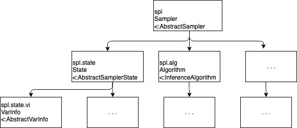
Turing implements AbstractMCMC's AbstractSampler with the Sampler struct defined in DynamicPPL. The most important attributes of an instance spl of Sampler are:
-
spl.alg: the sampling method used, an instance of a subtype ofInferenceAlgorithm -
spl.state: information about the sampling process, see below
When you call sample(mod, alg, n_samples), Turing first uses model and alg to build an instance spl of Sampler , then calls the native AbstractMCMC function sample(mod, spl, n_samples).
When you define your own Turing sampling method, you must therefore build:
-
a sampler constructor that uses a model and an algorithm to initialize an instance of
Sampler. For Importance Sampling:
function Sampler(alg::IS, model::Model, s::Selector)
    info = Dict{Symbol, Any}()
    state = ISState(model)
    return Sampler(alg, info, s, state)
end-
a state struct implementing
AbstractSamplerStatecorresponding to your method: we cover this in the following paragraph.
States
The vi field contains all the important information about sampling: first and foremost, the values of all the samples, but also the distributions from which they are sampled, the names of model parameters, and other metadata. As we will see below, many important steps during sampling correspond to queries or updates to spl.state.vi.
By default, you can use SamplerState, a concrete type defined in inference/Inference.jl, which extends AbstractSamplerState and has no field except for vi:
mutable struct SamplerState{VIType<:VarInfo} <: AbstractSamplerState
    vi :: VIType
end
When doing Importance Sampling, we care not only about the values of the samples but also their weights. We will see below that the weight of each sample is also added to spl.state.vi. Moreover, the average
of the sample weights is a particularly important quantity:
-
it is used to normalize the empirical approximation of the posterior distribution
-
its logarithm is the importance sampling estimate of the log evidence
To avoid having to compute it over and over again, is.jldefines an IS-specific concrete type ISState for sampler states, with an additional field final_logevidence containing
mutable struct ISState{V<:VarInfo, F<:AbstractFloat} <: AbstractSamplerState
    vi                 ::  V
    final_logevidence  ::  F
end

# additional constructor
ISState(model::Model) = ISState(VarInfo(model), 0.0)
The following diagram summarizes the hierarchy presented above.
2. Overload the functions used inside mcmcsample
A lot of the things here are method-specific. However Turing also has some functions that make it easier for you to implement these functions, for examples .
Transitions
AbstractMCMC stores information corresponding to each individual sample in objects called transition, but does not specify what the structure of these objects could be. You could decide to implement a type MyTransition for transitions corresponding to the specifics of your methods. However, there are many situations in which the only information you need for each sample is:
-
its value:
-
log of the joint probability of the observed data and this sample:
lp
Inference.jl defines a struct Transition, which corresponds to this default situation
struct Transition{T, F<:AbstractFloat}
    θ  :: T
    lp :: F
endHow sample works
A crude summary, which ignores things like parallelism, is the following:
sample calls mcmcsample, which calls
-
sample_init!to set things up -
step!repeatedly to produce multiple new transitions -
sample_end!to perform operations once all samples have been obtained -
bundle_samplesto convert a vector of transitions into a more palatable type, for instance aChain.
You can of course implement all of these functions, but AbstractMCMC as well as Turing also provide default implementations for simple cases. For instance, importance sampling uses the default implementations of sample_init! and bundle_samples, which is why you don’t see code for them inside is.jl.
3. Overload assume and observe
The functions mentioned above, such as sample_init!, step!, etc., must of course use information about the model in order to generate samples! In particular, these functions may need samples from distributions defined in the model, or to evaluate the density of these distributions at some values of the corresponding parameters or observations.
For an example of the former, consider Importance Sampling as defined in is.jl. This implementation of Importance Sampling uses the model prior distribution as a proposal distribution, and therefore requires samples from the prior distribution of the model. Another example is Approximate Bayesian Computation, which requires multiple samples from the model prior and likelihood distributions in order to generate a single sample.
An example of the latter is the Metropolis-Hastings algorithm. At every step of sampling from a target posterior
in order to compute the acceptance ratio, you need to evaluate the model joint density
with a sample from the proposal and the observed data.
This begs the question: how can these functions access model information during sampling? Recall that the model is stored as an instance m of Model. One of the attributes of m is the model evaluation function m.f, which is built by compiling the @model macro. Executing f runs the tilde statements of the model in order, and adds model information to the sampler (the instance of Sampler that stores information about the ongoing sampling process) at each step (see here for more information about how the @model macro is compiled). The DynamicPPL functions assume and observe determine what kind of information to add to the sampler for every tilde statement.
Consider an instance m of Model and a sampler spl, with associated VarInfo vi = spl.state.vi. At some point during the sampling process, an AbstractMCMC function such as step! calls m(vi, ...), which calls the model evaluation function m.f(vi, ...).
-
for every tilde statement in the
@modelmacro,m.f(vi, ...)returns model-related information (samples, value of the model density, etc.), and adds it tovi. How does it do that?-
recall that the code for
m.f(vi, ...)is automatically generated by compilation of the@modelmacro -
for every tilde statement in the
@modeldeclaration, this code contains a call toassume(vi, ...)if the variable on the LHS of the tilde is a model parameter to infer, andobserve(vi, ...)if the variable on the LHS of the tilde is an observation -
in the file corresponding to your sampling method (ie in
Turing.jl/src/inference/<your_method>.jl), you have overloadedassumeandobserve, so that they can modifyvito include the information and samples that you care about! -
at a minimum,
assumeandobservereturn the log densitylpof the sample or observation. the model evaluation function then immediately callsacclogp!!(vi, lp), which addslpto the value of the log joint density stored invi.
-
Here’s what assume looks like for Importance Sampling:
function DynamicPPL.assume(rng, spl::Sampler{<:IS}, dist::Distribution, vn::VarName, vi)
    r = rand(rng, dist)
    push!(vi, vn, r, dist, spl)
    return r, 0
end
The function first generates a sample r from the distribution dist (the right hand side of the tilde statement). It then adds r to vi, and returns r and 0.
The observe function is even simpler:
function DynamicPPL.observe(spl::Sampler{<:IS}, dist::Distribution, value, vi)
    return logpdf(dist, value)
end
It simply returns the density (in the discrete case, the probability) of the observed value under the distribution dist.
4. Summary: Importance Sampling step by step
We focus on the AbstractMCMC functions that are overridden in is.jl and executed inside mcmcsample: step!, which is called n_samples times, and sample_end!, which is executed once after those n_samples iterations.
-
During the -th iteration,
step!does 3 things:-
empty!!(spl.state.vi): remove information about the previous sample from the sampler’sVarInfo -
model(rng, spl.state.vi, spl): call the model evaluation function-
calls to
assumeadd the samples from the prior and tospl.state.vi -
calls to both
assumeorobserveare followed by the lineacclogp!!(vi, lp), wherelpis an output ofassumeandobserve -
lpis set to 0 afterassume, and to the value of the density at the observation afterobserve -
when all the tilde statements have been covered,
spl.state.vi.logp[]is the sum of thelp, i.e., the likelihood of the observations given the latent variable samples and .
-
-
return Transition(spl): build a transition from the sampler, and return that transition-
the transition’s
vifield is simplyspl.state.vi -
the
lpfield contains the likelihoodspl.state.vi.logp[]
-
-
-
When the,
n_samplesiterations are completed,sample_end!fills thefinal_logevidencefield ofspl.state-
it simply takes the logarithm of the average of the sample weights, using the log weights for numerical stability
-