Using Genie to visualize the action of a linear operator¶

The article is devoted to the application of GenieFramework for the development of an interactive web application demonstrating the action of a linear operator. As an example, we consider the transformation of a set of points representing a circle using a 2x2 matrix. The Stipple and PlotlyBase packages are used for implementation. The text describes in detail the key elements of the code with explanations following the relevant fragments. Special attention is paid to the justification of the use of reactive macros @in and @out to control the elements of the matrix (m11, m12, m21, m22), and the possibilities of using custom types, such as mutable struct, based on the Stipple documentation.

Application Concept¶

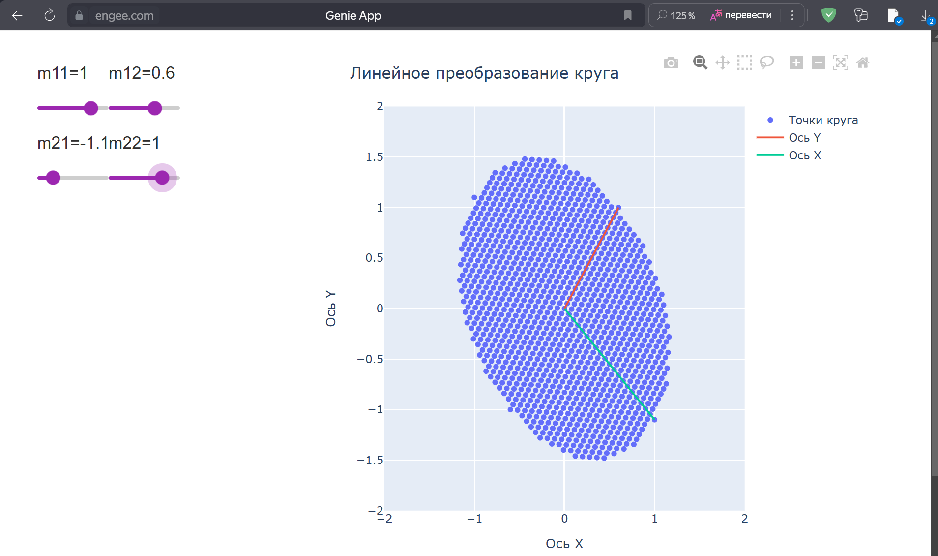
The appendix illustrates the effect of a 2x2 matrix as a linear operator on a two-dimensional set of points. Initially, the points form a circle of radius 1, and the user can change the elements of the matrix using sliders, observing the effects of transformations such as stretching, compression or rotation. This approach has educational potential by providing an interactive tool for learning linear algebra.

Creating a circle from a set of points¶

using GenieFramework, Stipple, Stipple.ReactiveTools, StippleUI, PlotlyBase

const circ_range = -1:0.05:1
const circle = [[i, j] for i in circ_range for j in circ_range if i^2 + j^2 <= 1]
const x_axis_points = findall(x -> x[1] == 0 &amp;&amp; x[2] >= 0, circle)
const y_axis_points = findall(x -> x[2] == 0 &amp;&amp; x[1] >= 0, circle)
const circle_matrix = Base.stack(circle)

This fragment forms the initial data for visualization. The range is defined circ_range -1 to 1 in increments of 0.05 for the x and y coordinates. Coordinate pairs are generated using the list inclusion. [i, j] filtered by the circle equation i^2 + j^2 <= 1, which gives a set of points approximating a circle of radius 1. The variables x_axis_points and y_axis_points They contain indexes of points lying on the positive parts of the Y and X axes, respectively, to highlight the basis vectors. Function Base.stack converts a list of coordinates into a matrix, where the first row is the x-coordinates and the second is the y—coordinates. Constants (const) are used for immutable data. The discrete step leads to some stepwise contour of the circle, but the method is simple to implement.

Developing a graph conversion function¶

function create_plot_data(m11::Float64, m12::Float64, m21::Float64, m22::Float64)
    transformed = [m11 m12; m21 m22] * circle_matrix
    [
scatter(x=transformed[1, :], y=transformed[2, :], mode=markers, name=Circle points),
        scatter(x=transformed[1, x_axis_points], y=transformed[2, x_axis_points], name=Y-axis),
scatter(x=transformed[1, y_axis_points], y=transformed[2, y_axis_points], name=X-axis, aspect_ratio=:equal)
    ]
end

const initial_plot_data = create_plot_data(1.0, 0.0, 0.0, 1.0)

Function create_plot_data responsible for converting points and preparing data for the graph. Accepts four arguments — elements of a 2x2 matrix (m11, m12, m21, m22). Performs matrix multiplication by circle_matrix, getting the new coordinates of the points in transformed. Returns an array of three objects scatter: all points of the circle, points on the Y-axis and points on the X-axis. Parameter aspect_ratio=:equal provides a uniform scale of the axes. The constant initial_plot_data sets the initial state of a graph with a unit matrix that does not change the circle.

Configuring the graph layout¶

const plot_layout = PlotlyBase.Layout(
    title=Linear circle transformation,
    xaxis=attr(title=X-axis, showgrid=true, range=[-2, 2]),
    yaxis=attr(title=Y-axis, showgrid=true, range=[-2, 2]),
    width=600, height=550
)

The fragment defines the graph layout using PlotlyBase.Layout. The heading, axis labels, grid, and value range from -2 to 2 are set. The graph dimensions are fixed: width 600 pixels, height 550 pixels. The layout is declared as a constant, as it does not change during the operation of the application.

Ensuring reactivity¶

@app begin
    @in m11 = 1.0
    @in m12 = 0.0
    @in m21 = 0.0
    @in m22 = 1.0
    @out plot_data = initial_plot_data
    @out plot_layout = plot_layout

    @onchange m11, m12, m21, m22 begin
        plot_data = create_plot_data(m11, m12, m21, m22)
    end
end

Block @app defines the reactive application model. Macros @in declare the matrix elements as input variables with initial values corresponding to the identity matrix. The macro @out sets the output data: plot_data for the schedule and plot_layout for the layout. The macro @onchange tracks changes in values m11, m12, m21, m22 and causes create_plot_data to update plot_data.

Customizing the user interface¶

function ui()
    sliders = [row([column([h6(m$(i)$(j)={{m$(i)$(j)}}), slider(-2:0.1:2, Symbol(m$(i)$(j)), color=purple)], size=3) for j in 1:2]) for i in 1:2]
    [
        row([
            column(sliders, size=4),
            column(plot(:plot_data, layout=:plot_layout))
        ], size=3)
    ]
end

@page(/, ui)

Function ui forms the interface. Variable sliders creates an array of two lines, each of which contains two sliders with captions (m11, m12, m21, m22). The range of sliders is from -2 to 2 in increments of 0.1. The interface consists of the line (row) with two columns: sliders on the left, a graph on the right, displayed via plot. The macro @page binds the interface to the root route /.

The need for application @in and @out¶

Reactivity in Stipple¶

Stipple implements a reactive model, providing synchronization of data and interface. Macros @in and @out integrate the elements into this model. @in binds data to interface elements (sliders), allowing the user to change them. @out updates the output data (graph) when the state changes. When using standard ads, for example m11 = 1.0 the interface elements lose their connection with the values, excluding their modification; @onchange it does not respond because Stipple does not track such data; interactivity is disrupted because values are not passed to JavaScript.

An alternative with custom types¶

According to the Stipple documentation (Types of variables in Stipple) , it is possible to use mutable struct as reactive variables:

mutable struct MatrixState
    m11::Float64
    m12::Float64
    m21::Float64
    m22::Float64
end

@app begin
    @in state = MatrixState(1.0, 0.0, 0.0, 1.0)
    @out plot_data = initial_plot_data
    @out plot_layout = plot_layout

    @onchange state begin
        plot_data = create_plot_data(state.m11, state.m12, state.m21, state.m22)
    end
end

Structure MatrixState announced via @in, which allows Stipple to track changes in its fields. However, in this application, preference is given to individual variables (@in m11 etc.), as this simplifies the management of matrix elements through separate sliders.

Without @in and @out The matrix elements remain isolated in Julia, without interacting with the interface. Reactive macros or mutable struct with @in/@out They provide the necessary communication, and the choice of approach depends on the data structure and interface requirements.

To launch the application, we will use the one already familiar from previous статьям by construction:

Conclusion¶

The article demonstrates the use of GenieFramework to create an interactive application that visualizes the action of a linear operator. Reactive macros @in and @out we have provided a link between the interface and logic, and the possibility of using mutable struct provides flexibility for complex scenarios. The app highlights Genie's capabilities for developing educational tools.---