Modeling of the electrocardiosignal

The example shows the modeling of an electrocardiosignal based on asymmetric Gaussian functions, including the formation of a normal signal and a number of pathological changes.

Workspace preparation and visualization settings

Function engee.clear() cleans up workspaces:

engee.clear()

Warning: detected a stack overflow; program state may be corrupted, so further execution might be unreliable.

Two graph rendering modes are available to visualize the results.:

For static, fast rendering, use gr().
For interactive, dynamic visualization with the ability to scale and view values, use plotlyjs().

Select one of the commands by commenting out the second one. Both backends are mutually exclusive, and the last one called will be activated.

gr()
# plotlyjs()

Plots.GRBackend()

Electrocardiogram signal

The figure below shows two consecutive cardiac cycles and the basic elements of a normal electrocardiogram.

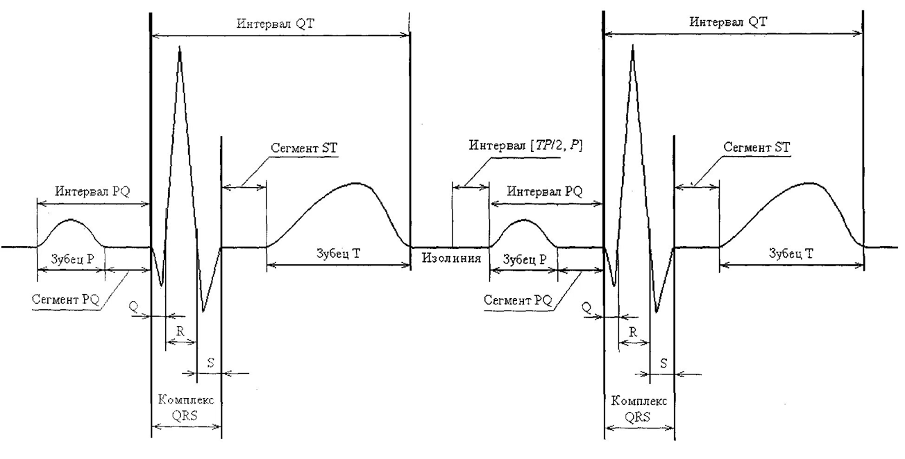
This figure shows the main elements of a normal ECG and their place within a single cardiac cycle. The P wave reflects the spread of arousal through the atria. It is followed by the segment PQ, which corresponds to the conduction of the pulse through the atrioventricular junction, and the interval PQ covers the entire path from the beginning of atrial excitation to the beginning of ventricular excitation. The QRS complex reflects ventricular depolarization: ** the Q wave** corresponds to the initial excitation of the interventricular septum, the R wave corresponds to the spread of excitation through the bulk of the ventricular myocardium, and the S wave corresponds to the final stage of depolarization in the basal ventricles. After the QRS complex, the ST segment is located, which corresponds to the period of complete coverage of the ventricular myocardium by excitation and is normally located close to the isoline. This is followed by the T wave, reflecting ventricular repolarization. The QT interval covers the area from the beginning of the QRS complex to the end of the T wave and characterizes the total time of depolarization and repolarization of the ventricles, including depolarization and subsequent repolarization.

This representation of the ECG is convenient for further mathematical modeling, since it allows us to consider the cardiocycle as a sequence of separate informative fragments, each of which can be described and parameterized independently.

Description of the model

In this example, we consider the modeling of an electrocardiosignal based on the sum of asymmetric Gaussian functions. This approach allows us to represent a single cardiac cycle as a collection of individual fragments. In the implementation used, the signal is formed from the components , , , , and moreover, there are two components and They are used for a more flexible description of the complex. . The model is based on the representation of a signal as a sum of individual waves.:

where is the parameter determines the amplitude -th component, parameter sets the position of its time extremum, and the function It is responsible for the width of the wave to the left and right of the extreme point. In order for the same function to describe both symmetric and non-symmetric signal fragments, the width is set piecewise.:

If , the corresponding wave is symmetric, and if then it becomes asymmetrical. It is this property that allows you to flexibly set the shape of individual ECG sections and obtain a more realistic morphology of the signal.

The implementation of this model is based on two functions. The first function forms one non-symmetrical Gaussian component of the signal. If we denote such a component by , then it is written as:

In the code, this idea is implemented by a function asym_gauss, which checks for each point on the time axis whether it is to the left or to the right of the point , and depending on this , uses either the left width , or the right width . Thus, the same function can describe both positive and negative waves, as well as both symmetrical and asymmetric fragments of the electrocardiosignal.

The second function is intended to ecg_complex to form the entire cardiac cycle. It summarizes several components, each of which is calculated by the same function. asym_gauss, but with its own set of parameters. In its expanded form, this formula has the form:

function asym_gauss(t, A, mu, b1, b2)
    y = zeros(length(t))

    for i in 1:length(t)
        if t[i] <= mu
            y[i] = A * exp(-((t[i] - mu)^2) / (2 * b1^2))
        else
            y[i] = A * exp(-((t[i] - mu)^2) / (2 * b2^2))
        end
    end

    return y
end

function ecg_complex(t, A, mu, b1, b2)
    y = zeros(length(t))

    for k in 1:length(A)
        y += asym_gauss(t, A[k], mu[k], b1[k], b2[k])
    end

    return y
end

ecg_complex (generic function with 1 method)

Simulation of a normal electrocardiosignal

To simulate the signal, we will set a sampling frequency of 1 kHz. With this value, the time step is 1 ms. Next, the time axis of one cardiac cycle with a duration of 1 second is formed.

fs = 1e3
Ts = 1/fs
t = 0:Ts:1-Ts

0.0:0.001:0.999

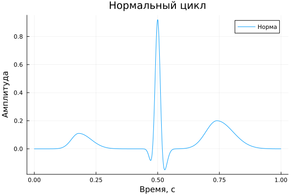
In this part of the example, the parameters of a normal electrocardiosignal are set and its formation is performed. Arrays , , and The amplitudes of the components, the positions of their time extremes, as well as the widths on the left and right, which determine the shape and asymmetry of individual waves, are determined. After that, using the function ecg_complex One normal heart cycle is formed, which is then displayed on the graph. The received signal is used as a basic option for subsequent comparison with pathological forms of ECS.

A_norm  = [ 0.11, -0.11, 0.95, 0.02, -0.18, 0.00, 0.20 ]
mu_norm = [ 0.18,  0.476, 0.500, 0.510, 0.523, 0.60, 0.74 ]
b1_norm = [ 0.03,  0.010, 0.010, 0.006, 0.012, 0.040, 0.045 ]
b2_norm = [ 0.05,  0.010, 0.010, 0.007, 0.014, 0.040, 0.065 ]

y_norm = ecg_complex(t, A_norm, mu_norm, b1_norm, b2_norm)

p1 = plot(t, y_norm,
    xlabel = "Time, from",
    ylabel = "The amplitude",
    title = "The normal cycle",
    label = "Standard"
)

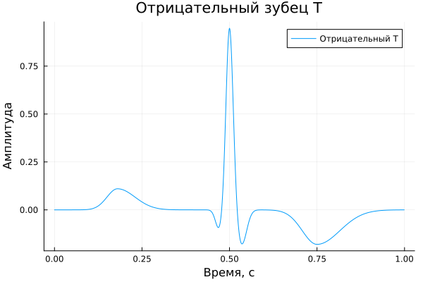
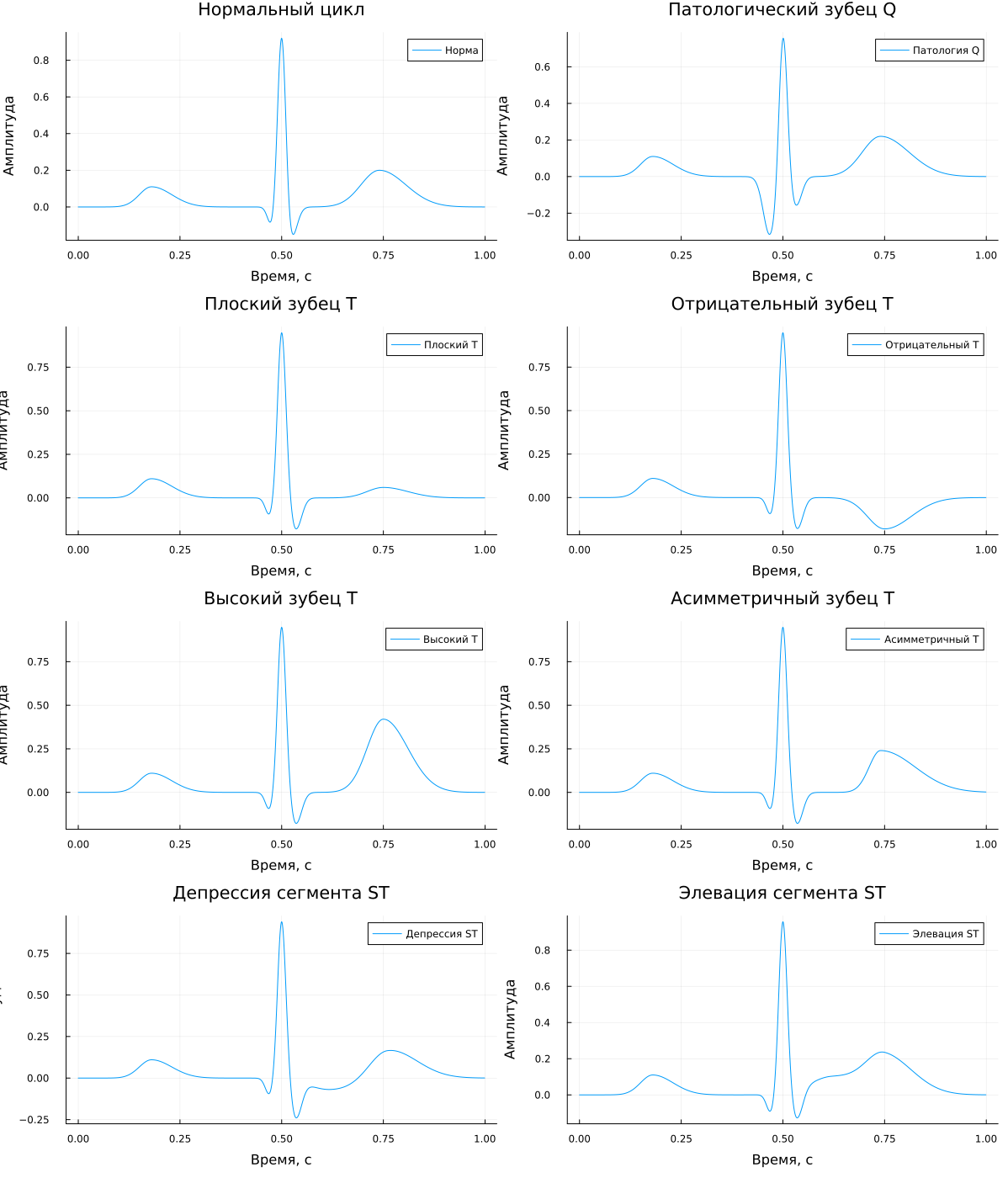
After forming a normal signal, the model is used to simulate pathological changes in the ECS. In this example, the pathological tooth is considered. , flat, negative, high and asymmetrical prong , as well as depression and segment elevation . Each option is obtained by changing the parameters of the corresponding components without changing the overall structure of the model.

Modeling of electrocardiosignal pathologies

This part examines the modeling of pathological changes in the electrocardiosignal based on a parametric model of the cardiac cycle. By changing the amplitudes, time positions, and widths of the individual signal components, it is possible to reproduce the characteristic deviations of the ECG shape without changing the overall structure of the model.

As part of the example, the following variants of pathological changes are considered:

pathological Q wave;
Flat T-prong;
Negative T-prong;
High T-prong;
Asymmetric T-prong;
ST segment depression;
Elevation of the ST segment.

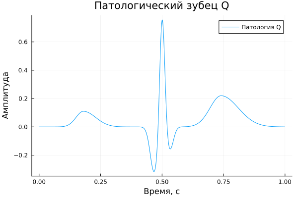
Pathological Q wave

A_q  = [ 0.11, -0.32, 0.82, 0.03, -0.16, 0.00, 0.22 ]
mu_q = [ 0.18,  0.468, 0.500, 0.512, 0.532, 0.60, 0.74 ]
b1_q = [ 0.03,  0.016, 0.010, 0.006, 0.012, 0.040, 0.045 ]
b2_q = [ 0.05,  0.018, 0.010, 0.007, 0.014, 0.040, 0.070 ]

y_q = ecg_complex(t, A_q, mu_q, b1_q, b2_q)

p2 = plot(t, y_q,
    xlabel = "Time, from",
    ylabel = "The amplitude",
    title = "Pathological Q wave",
    label = "Pathology of Q"
)

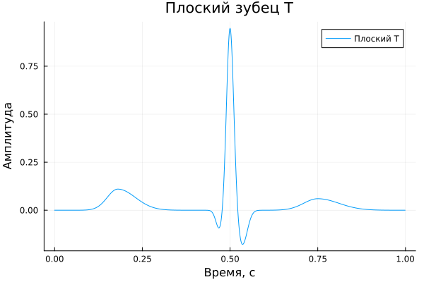
Flat tooth T

A_flatT  = [ 0.11, -0.10, 0.95, 0.03, -0.18, 0.00, 0.06 ]
mu_flatT = [ 0.18,  0.470, 0.500, 0.515, 0.535, 0.60, 0.75 ]
b1_flatT = [ 0.03,  0.010, 0.010, 0.006, 0.012, 0.040, 0.040 ]
b2_flatT = [ 0.05,  0.010, 0.010, 0.007, 0.014, 0.040, 0.060 ]

y_flatT = ecg_complex(t, A_flatT, mu_flatT, b1_flatT, b2_flatT)

p3 = plot(t, y_flatT,
    xlabel = "Time, from",
    ylabel = "The amplitude",
    title = "Flat tooth T",
    label = "Flat T"
)

Negative T-wave

A_negT  = [ 0.11, -0.10, 0.95, 0.03, -0.18, 0.00, -0.18 ]
mu_negT = [ 0.18,  0.470, 0.500, 0.515, 0.535, 0.60, 0.75 ]
b1_negT = [ 0.03,  0.010, 0.010, 0.006, 0.012, 0.040, 0.042 ]
b2_negT = [ 0.05,  0.010, 0.010, 0.007, 0.014, 0.040, 0.065 ]

y_negT = ecg_complex(t, A_negT, mu_negT, b1_negT, b2_negT)

p4 = plot(t, y_negT,
    xlabel = "Time, from",
    ylabel = "The amplitude",
    title = "Negative T-wave",
    label = "Negative T"
)

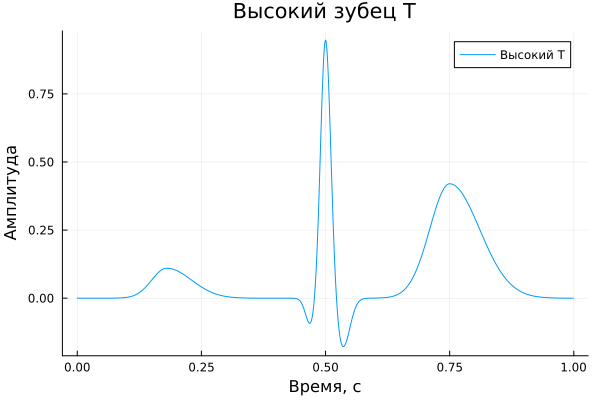
High T-prong

A_highT  = [ 0.11, -0.10, 0.95, 0.03, -0.18, 0.00, 0.42 ]
mu_highT = [ 0.18,  0.470, 0.500, 0.515, 0.535, 0.60, 0.75 ]
b1_highT = [ 0.03,  0.010, 0.010, 0.006, 0.012, 0.040, 0.040 ]
b2_highT = [ 0.05,  0.010, 0.010, 0.007, 0.014, 0.040, 0.060 ]

y_highT = ecg_complex(t, A_highT, mu_highT, b1_highT, b2_highT)

p5 = plot(t, y_highT,
    xlabel = "Time, from",
    ylabel = "The amplitude",
    title = "High T-prong",
    label = "High T"
)

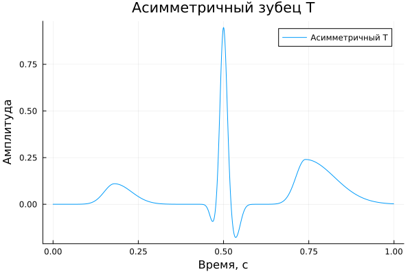
The asymmetric T-prong

A_asymT  = [ 0.11, -0.10, 0.95, 0.03, -0.18, 0.00, 0.24 ]
mu_asymT = [ 0.18,  0.470, 0.500, 0.515, 0.535, 0.60, 0.74 ]
b1_asymT = [ 0.03,  0.010, 0.010, 0.006, 0.012, 0.040, 0.028 ]
b2_asymT = [ 0.05,  0.010, 0.010, 0.007, 0.014, 0.040, 0.085 ]

y_asymT = ecg_complex(t, A_asymT, mu_asymT, b1_asymT, b2_asymT)

p6 = plot(t, y_asymT,
    xlabel = "Time, from",
    ylabel = "The amplitude",
    title = "The asymmetric T-prong",
    label = "The asymmetric T"
)

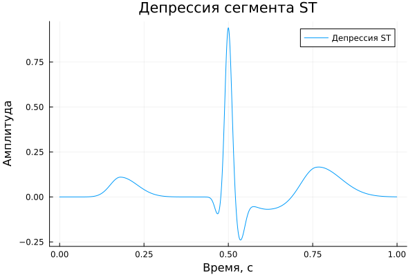
ST segment depression

A_depST  = [ 0.11, -0.10, 0.95, 0.03, -0.22, -0.07, 0.18 ]
mu_depST = [ 0.18,  0.47, 0.50, 0.515, 0.535, 0.62, 0.76 ]
b1_depST = [ 0.03,  0.010, 0.010, 0.006, 0.012, 0.055, 0.045 ]
b2_depST = [ 0.05,  0.010, 0.010, 0.007, 0.014, 0.080, 0.070 ]

y_depST = ecg_complex(t, A_depST, mu_depST, b1_depST, b2_depST)

p7 = plot(t, y_depST,
    xlabel = "Time, from",
    ylabel = "The amplitude",
    title = "ST segment depression",
    label = "ST Depression"
)

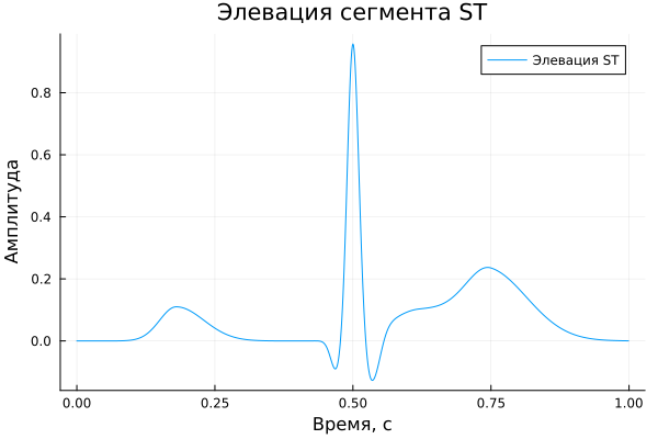
ST segment elevation

A_eleST  = [ 0.11, -0.10, 0.95, 0.03, -0.16, 0.10, 0.20 ]
mu_eleST = [ 0.18,  0.47, 0.50, 0.515, 0.535, 0.62, 0.75 ]
b1_eleST = [ 0.03,  0.010, 0.010, 0.006, 0.012, 0.055, 0.045 ]
b2_eleST = [ 0.05,  0.010, 0.010, 0.007, 0.014, 0.090, 0.070 ]

y_eleST = ecg_complex(t, A_eleST, mu_eleST, b1_eleST, b2_eleST)

p8 = plot(t, y_eleST,
    xlabel = "Time, from",
    ylabel = "The amplitude",
    title = "ST segment elevation",
    label = "ST Elevator"
)

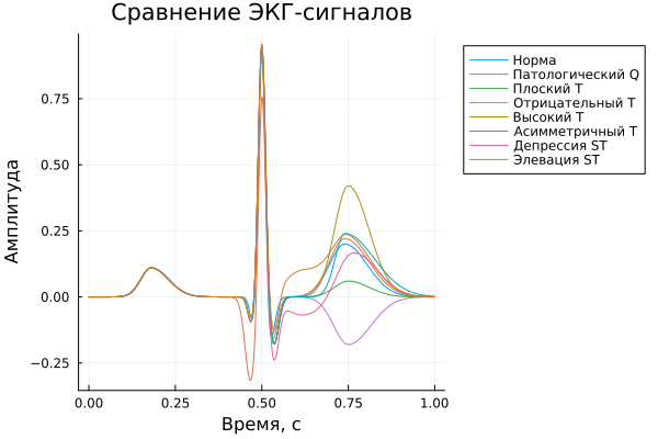
Comparison of normal and pathological EX

In this part, a comparison of normal and pathological ECS variants is performed. For clarity, the results are presented in two versions: in the first case, all the signals are displayed on one common graph, which allows you to evaluate the differences in shape and the mutual displacement of individual sections; in the second case, each signal is displayed on a separate plot area using the layout layout = (4, 2), which makes it more convenient to examine each pathology in detail.

plot(t, y_norm, 
    xlabel="Time, from", 
    ylabel="The amplitude", 
    title="Comparison of ECG signals", 
    label="Standard",
    legend_position = :outertopright
)

plot!(t, y_q, label="Pathological Q")
plot!(t, y_flatT, label="Flat T")
plot!(t, y_negT, label="Negative T")
plot!(t, y_highT, label="High T")
plot!(t, y_asymT, label="The asymmetric T")
plot!(t, y_depST, label="ST Depression")
plot!(t, y_eleST, label="ST Elevator")

Let's display all the signals separately using layout = (4, 2).

plot(    p1, p2, p3, p4, p5, p6, p7, p8,
    layout = (4, 2),
    size = (1200, 1400)
)

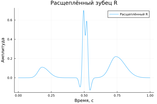
Split prong R

Earlier, two prong components were introduced when describing the model - and . However, in the previously discussed examples, such a case was not analyzed separately. In this regard, we will further consider it separately and simulate an electrocardiosignal with a split tooth. .

A_splitR  = [ 0.11, -0.10, 0.70, 0.62, -0.16, 0.00, 0.22 ]
mu_splitR = [ 0.18,  0.47, 0.495, 0.520, 0.538, 0.61, 0.74 ]
b1_splitR = [ 0.03,  0.010, 0.008, 0.008, 0.012, 0.045, 0.045 ]
b2_splitR = [ 0.05,  0.010, 0.009, 0.009, 0.014, 0.045, 0.070 ]

y_splitR = ecg_complex(t, A_splitR, mu_splitR, b1_splitR, b2_splitR)

p9 = plot(t, y_splitR,
    xlabel = "Time, from",
    ylabel = "The amplitude",
    title = "Split prong R",
    label = "Split R"
)

Conclusion

In this example, parametric modeling of an electrocardiosignal based on the sum of asymmetric Gaussian functions was considered. It is shown that this approach makes it possible to form one cycle of an electrocardiosignal as a set of separate informative components and flexibly control its shape by changing the amplitudes, time positions and widths of the corresponding waves.