Averaging of closely spaced points within a tolerance

Let's show how you can reduce the number of points on the graph, leaving only those that differ from the rest by some criterion.

Initial data

Let's use the function from the file peaks.jl, which will create a smooth surface with several protrusions in the range [-3.3], [-3.3]. Let's add some noise along the Z axis to the data. Now the point cloud no longer lies on one surface, but is scattered around it.

Pkg.add(["Statistics", "GroupSlices"])

gr( format=:png ) # Обратите внимание, теперь все графики, в рамках
                  # текущей рабочей сессии, будут выводиться в PNG

include( "$(@__DIR__)/peaks.jl" );

xy = rand(10000, 2) .* 6 .- 3; 
z = peaks.( xy[:,1], xy[:,2] ) .+ 0.5 .- rand(10000,1);
A = [xy z]

scatter( A[:,1], A[:,2], A[:,3], camera=(45, 20), ms=2, markerstrokewidth=0.1, leg=false )

Restoring a smooth surface

Inside this point cloud, we will look for those points that could be combined according to the following criteria:

the distance between the points does not exceed tol.
we are not interested in the Z axis, we compare only X and Y.

tol = 0.33;

To identify identical areas, we round off the original data set by rounding all the coordinates of each point to an integer, first multiplying by 1/tol.

aA = round.( (1/tol) .* A[:,1:2], digits=0);

Our matrix now consists of a large number of groups of vectors with identical values. How do we group them? You can compare vectors piecemeal with each other, but in a shorter way.

This operation can be performed using the function groupslices from the library GroupSlices (if necessary, to set it, uncomment and execute the following cell):

#]add GroupSlices

using GroupSlices
C = groupslices( aA, dims=1 );

Function groupslices for each row r of the matrix, returns the index *of the first encountered row identical to r.

Let's average the points in each subgroup.

using Statistics
avgA = [  mean( A[C .== c, :], dims=1) for c in unique( C ) ]
avgA = vcat( avgA... ); # Мы получили матрицу из матриц; осуществим вертикальную конкатенацию строчек

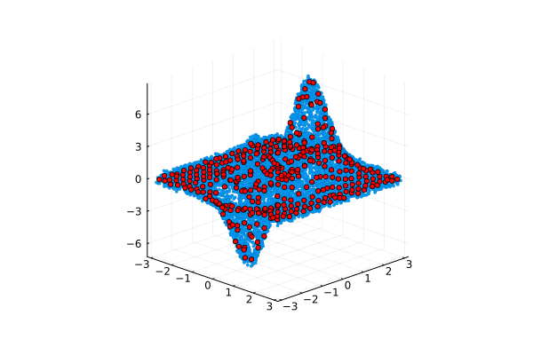
Now we can build a graph from the averaged points, noting for ourselves that although the data set has not become structured, we have got rid of the variability along the Z axis, preserving the general appearance of the source data.

scatter( A[:,1], A[:,2], A[:,3], camera=(45, 20), ms=2, markerstrokewidth=0.1, leg=false )
scatter!( avgA[:,1], avgA[:,2], avgA[:,3], color=:red, ms=3, legend=false )

Individual areas can be seen by coloring them as follows:

scatter( A[:,1], A[:,2], A[:,3], camera=(45, 20), ms=2, markerstrokewidth=0.1, leg=false, zcolor=C./maximum(C), c=:prism )
scatter!( avgA[:,1], avgA[:,2], avgA[:,3], color=:white, ms=3, legend=false, camera=(0,90) )

Conclusion

We filtered out the noisy function by selecting some unique points. In selecting them, we relied on the acceptable proximity between the reference points along the X and Y axes.