Construction of a vector diagram of an asynchronous motor

This example shows the construction of a rotating vector diagram of an asynchronous motor with a closed-loop rotor (ADKZ) for one phase in static mode.

Introduction

The ADKZ vector diagram illustrates the relationship of the main flow vectors, motor voltages and currents in statics. During engine operation, all vectors rotate in the cross-sectional plane around the axis of rotation of the rotor, while their modules and phase shifts change.

In this calculation, a diagram is constructed for the phase A of the engine in steady state (the lengths and phases of the vectors do not change). The modules and phases of the vectors are calculated based on the substitution scheme calculated in the example according to the passport data of the MTK011-6 crane-metallurgical engine.

Engine calculation

We will determine the initial data based on the passport data of the ADKZ in question.:

# Passport data of the MTK011-6 engine
Pₙ = 1400; Uₙ = 380; f₁ = 50;           # Rated power [W], line voltage [V], frequency [V]
nₙ = 870; p = 3; η = 0.72;              # Rated rotation speed [rpm], number of pole pairs, efficiency
cosϕ = 0.69; Iₙ = 4.8; I₀ = 3.2;        # Rated power factor, rated current [A], no-load current [A]
ki = 3; mₚ = 2.8; mₘ = 2.8; J = 0.02;   # Coefficients of maximum current, starting and maximum torque, moment of inertia of the motor [kg·m2]

Now let's move on to calculating the parameters of the ADKZ replacement scheme.:

# Calculation of substitution scheme parameters
U₁ = Uₙ/sqrt(3);                           # Rated phase voltage of the stator [V]
n₀ = 60*f₁/p;                             # Synchronous rotation speed [rpm]
sₙ = (n₀-nₙ)/n₀; sₖ = sₙ*(mₘ+sqrt(mₘ^2-1)); # Nominal and critical slip
ω₀ = 2π*f₁/p; ωₙ = π*nₙ/30;                # Synchronous and nominal angular velocity of the rotor [rad/s]
Mₙ = Pₙ/ωₙ; Mₘ = Mₙ*mₘ; Mₚ = Mₙ*mₚ;           # Nominal, maximum and starting torque [Nm]
pₘ = 0.05*Pₙ;                              # Mechanical losses (5% of Pₙ) [W]
C = 0.8093072740472634;                   # Constructive coefficient (preliminary)

R₂ = 1/3*(Pₙ+pₘ)/(Iₙ^2*(1-sₙ)/sₙ);              # The reduced active resistance of the rotor winding is [Ohms]
R₁ = U₁*cosϕ*(1-η)/Iₙ - C^2*R₂ - pₘ/(3*Iₙ^2);  # Active resistance of the stator winding [Ohms]

L₁σ = L₂σ = U₁/(4π*f₁*(1+C^2)*ki*Iₙ);          # Stator dissipation inductance and reduced rotor [Gn]
L₁ = L₂ = U₁/(2π*f₁*Iₙ*sqrt(1-cosϕ^2)-2/3*(2π*f₁*Mₘ*sₙ)/(p*U₁*sₖ)); # Stator inductance and reduced rotor [Gn]
Lm = L₁ - L₁σ;                                 # Magnetic circuit inductance [Gn]

C = 1 + L₁σ/Lm                             # Constructive coefficient (specified)

X₁σ = 2π*f₁*L₁σ;    X₂σ = 2π*f₁*L₂σ        # Reactive resistances of stator dissipation and reduced rotor [Ohms]

I₂ = U₁/hypot(R₁+R₂*(1+(1-sₙ)/sₙ), X₁σ+X₂σ) # Rotor current [A] (preliminary value)
ψ₂ = atan(X₂σ*sₙ/R₂);                       # Rotor current delay angle [rad] (to rotor EMF, preliminary value)

For further calculations and construction, we turn to the complex representation of currents and voltages. Auxiliary functions must first be defined.

Auxiliary functions

The following function allows you to concisely prepare the area of the vector diagram in the future.

"""
    coordinateplane(header::String, length_ axis)

A function for plotting coordinate axes.
Plots, GR backend.
Gets the value of the title attribute and the length of the axis (X or Y)
The scale of the axes is the same, the labels of the graphs are at the top left
"""
function coordinateplane(header::String, length_ axis)
    gr()
    plot(size=(500, 500), legend=:topleft, aspect_ratio=:equal,
        xlabel="The X-axis", ylabel="The Y axis",
        title=title, showaxis = false)
    quiver!([-длина_оси/2], [0], quiver=([длина_оси], [0]), color=:grey, width = 2) # The X-axis
    quiver!([0], [-длина_оси/2], quiver=([0], [длина_оси]), color=:grey, width = 2) # The Y axis
end;

The following function combines instructions for preprocessing complex vectors - scaling and rotation, as well as constructing a complex vector relative to the previous one.

"""
    vectorplot(initial::ComplexF64, the resulting::ComplexF64,
               цвет::Symbol=:black, лэйбл::String="")

A function for constructing the resulting vector starting from the initial one.
Plots, GR backend.
Gets the complex values of the initial and resulting vectors, the color and label attributes of the resulting vector.
The rotation and multiplier attributes are used to rotate the resulting vector by a given angle [rad] and scale accordingly.
It is recommended to execute coordinateplane() before using it.
"""
function vectorplot(начальный::ComplexF64, результирующий::ComplexF64, цвет::Symbol=:black, лэйбл::String="", поворот=0.0, множитель=1.0)
    начальный = начальный*множитель*exp(поворот*im)             # Rotate and zoom
    результирующий = результирующий*множитель*exp(поворот*im)   # Rotate and zoom
    Plots.quiver!([real(initial)], [imag(initial)], quiver=([real(resultant)], [imag(resultant)]), color=color, label=label)
end;

Construction of a vector diagram of currents

Let's define complex vectors of currents:

Ȯ = 0.0 + 0.0*im                # Zero is the vector at the origin
İ₀ = I₀ + 0.0*im                # Complex no-load current. The active component is assumed to be 0.0 [A]
İ₂ = I₂*exp((3π/2-ψ₂)*im)       # Complex rotor current [A]
İ₁ = İ₀ - İ₂;                   # Complex stator current [A]

Let's construct a vector diagram of the currents:

coordinateplane("Vector diagram of asynchronous motor currents", 20)

vectorplot(Ȯ,   İ₀,     :blue,     "İ₀, [A]")
vectorplot(İ₀,  -İ₂,    :green,    "-İ₂, [A]")
vectorplot(Ȯ,   İ₁,     :red,      "İ₁, [A]")
vectorplot(Ȯ,   İ₂,     :magenta,  "İ₂, [A]")

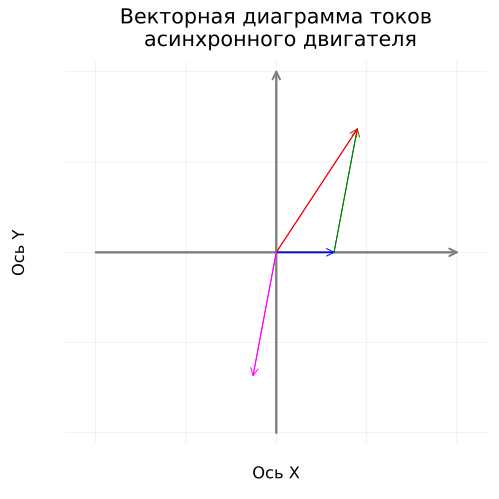
The general appearance of the diagram, as well as the location of the vectors relative to each other and on the plane, correspond to expectations. Let's move on to specifying the parameters of the vectors and constructing a vector stress diagram.

Construction of a vector stress diagram

Let's define the complex voltage and EMF vectors:

Ż₁ = R₁ + X₁σ*im        # Total integrated resistance of the stator circuit [V]
Ů₁_r = İ₁*R₁            # Active voltage drop in the stator circuit [V]
Ů₁_x = İ₁*X₁σ*im        # Reactive voltage drop in the stator circuit [V]
Ů₁_z = İ₁*Ż₁            # Total voltage drop in the stator circuit [V]

Ů₁ = U₁*im              # Complex supply voltage [V]
Ė₁ = Ė₂ = Ů₁_z - Ů₁;    # Stator EMF and reduced rotor [V]

Let's specify the location on the plane and the parameters of the complex vectors:

Ė₁ = Ė₂ = abs(Ė₁)*exp(-π/2*im)     # EMF of the stator and the reduced rotor [In] (shifted along the complex axis)
Ů₁ = -Ė₁ + Ů₁_z                    # Supply voltage [V] (taking into account the rotation of the EMF vector)

I₂ = abs(Ė₂)/hypot((R₂/sₙ), X₂σ)    # Reduced rotor current modulus [A] (specified value)
ψ₂ = atan(X₂σ*sₙ/R₂)                # Rotor current delay angle [rad] (specified value)
İ₂ = I₂*exp((3π/2-ψ₂)*im)          # Reduced complex rotor current [A]

İ₁ = İ₀ - İ₂                       # Complex stator current [A] (specified)

Ů₂_r = İ₂*(R₂ + R₂*(1-sₙ)/sₙ)       # The reduced active voltage drop in the rotor circuit [V]
Ů₂_x = İ₂*X₂σ*im;                  # Reduced reactive voltage drop in the rotor circuit [V]

Let's construct a vector diagram of ADKZ stresses:

coordinateplane("Vector diagram of asynchronous motor voltages", 500)

vectorplot(Ȯ,        -Ė₁,   :green,   "-Ė,, [In]")
vectorplot(-Ė₁,      Ů₁_r,  :blue,    "Ů₁_r, [In]")
vectorplot(-Ė₁+Ů₁_r, Ů₁_x,  :orange,  "Ů₁_x, [In]")
vectorplot(-Ė₁,      Ů₁_z,  :purple,  "Ů₁_z, [In]")
vectorplot(Ȯ,        Ů₁,    :red,     "Ů₁, [In]")
vectorplot(Ȯ,        Ė₁,    :magenta, "Ė,, [In]")
vectorplot(Ȯ,        Ů₂_r,  :blue,    "Ů₂_r, [In]")
vectorplot(Ů₂_r,     Ů₂_x,  :orange,  "Ů₂_x, [In]")

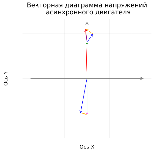
The voltage diagram also corresponds to the expected parameters. Finally, we will construct a complete diagram of currents and voltages rotating in a complex plane.

Building a rotating vector diagram

Setting the rotation cycle that will be animated.
We will scale the current vectors for clarity.

RotateDiagram = @animate for δ in range(0.0, step=2π/100, length = 100)
    coordinateplane("Vector diagram of an asynchronous motor", 500)

    vectorplot(Ȯ,  İ₀,  :blue,    "İ₀·15, [A]",  δ, 15)
    vectorplot(İ₀, -İ₂, :green,   "-İ₂·15, [A]", δ, 15)
    vectorplot(Ȯ,  İ₁,  :red,     "İ₁·15, [A]",  δ, 15)
    vectorplot(Ȯ,  İ₂,  :magenta, "İ₂·15, [A]",  δ, 15)

    vectorplot(Ȯ,           -Ė₁,  :green,   "-Ė,, [In]",   δ)
    vectorplot(-Ė₁,         Ů₁_r, :blue,    "Ů₁_r, [In]",  δ)
    vectorplot((-Ė₁+Ů₁_r),  Ů₁_x, :orange,  "Ů₁_x, [In]",  δ)
    vectorplot(-Ė₁,         Ů₁_z, :purple,  "Ů₁_z, [In]",  δ)
    vectorplot(Ȯ,           Ů₁,   :red,     "Ů₁, [In]",    δ)
    vectorplot(Ȯ,           Ė₁,   :magenta, "Ė,, [In]",    δ)
    vectorplot(Ȯ,           Ů₂_r, :blue,    "Ů₂_r, [In]",  δ)
    vectorplot(Ů₂_r,        Ů₂_x, :orange,  "Ů₂_x, [In]",  δ)
end

gif(RotateDiagram, "RotateDiagram.gif", fps = 20)

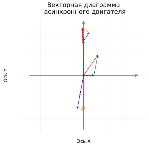
[ Info: Saved animation to /user/alexevs/_new/induction_motor_vector_diagram/RotateDiagram.gif

It should be noted that the rotation frequency of the vectors in the diagram has been reduced to allow rotation analysis by 250 times (from 50 to 1/5 Hz).

Conclusion

As a result of the script, we have obtained a rotating vector diagram of ADKZ currents and voltages rotating in a complex plane. Further possible extensions of this example include clarifying the calculation of the substitution scheme and vectors, constructing a diagram in dynamic mode (load regulation, acceleration or deceleration), and constructing a diagram for three phases - symmetrical and asymmetrical.

List of used literature

Voldek A.I. Electric machines. Textbook for students of higher engineering institutions. - 3rd ed., reprint. - L.: Energiya, 1978. - 832 p., ill.
Vyoshenevsky S.N. Characteristics of motors in an electric drive - 6th ed., ispr. - M.: Energy, 1977. - 431 p., ill.