Views as a way to improve code performance
This script discusses the use of views, a mechanism that allows accessing array elements without creating copies of them.
Topics will be covered:
- the difference between a slice copy (slicing) and a view (view)
- the use of macros
@viewand@viewsand their differences.
In order to test the effectiveness of using views, we will connect the benchmark libraries.
import Pkg; Pkg.add("BenchmarkTools")
The problem of copying
When we use syntax b = a[1:5], then b becomes a copy of the first five elements a, rather than "linking by address" to the elements a.
a = collect(1:10)
b = a[1:5]           # [1, 2, 3, 4, 5]
println(pointer(a))
println(pointer(b))
b .= 0               # [0, 0, 0, 0, 0]
a'                   # как видим, матрица не поменялась, что и логично
To change our original vector, we have to do an extra action.:
a[1:5] .= b[1:5]
a'
The view function
Representations just allow you to use the usual syntax, but not to create copies, but to access directly to the "memory cells" of arrays.
To do this, you can use the function view
a = collect(1:10000)
# '÷' is not the same as '/' (÷ = div())
view_of_a = view(a,1:length(a)÷2) # The end won't work here.
view_of_a .= 0
a
pointer(view_of_a) == pointer(a)
Let's make sure that using views allows us to avoid allocating extra memory for copies by using @allocated, showing the number of allocated bytes.
println(@allocated (subarray_of_a = a[1:end÷2]))
println(@allocated (view_of_a = view(a,1:length(a)÷2)))
@view
But using the function view it does not correspond to the above statement about the "familiar interface", since we could not use, for example, the keyword end.
You can use a macro to solve this problem. @view:
a = repeat(1:10,inner=3)
b = @view a[end-3:end]
b .= 0
a'
But the question may arise: why do we need extra variables when you can just do
a = repeat(1:10,inner=3)
a[end-3,3] .= 0
The answer to this can be formulated as follows:
Views are needed as a combination of efficient use of resources and maintaining code readability.
Suppose there is a task to output and calculate the sum of a triplet of elements.
for i in 0:(length(a)÷3-1)
    println("sum of $(a[3i+1:3i+3]) -> $(sum(a[3i+1:3i+3]))")
end
It can be seen that there are duplicate elements, and it is also easy to make a mistake in one of the indexes.
for i in 0:(length(a)÷3-1)
    triplet = a[3i+1:3i+3]
    println("sum of $triplet -> $(sum(triplet))")
end
In addition, we can see that a function that uses representations will allocate much less memory and run significantly faster.
To do this, we will use the macro @btime, showing the execution time of the function and the memory allocated at the same time, running the function several times and averaging the values.
(The output to the console was removed from the functions so as not to clog up the console during multiple function calls)
using BenchmarkTools

function tripletssum_subarray(v)
for i in 0:(length(v)÷3-1)
    triplet = v[3i+1:3i+3]
end
end

function tripletssum_view(v)
for i in 0:(length(v)÷3-1)
    triplet = @view v[3i+1:3i+3]
end
end


a = repeat(1:10000,inner=3)

println(@btime tripletssum_subarray(a))
println(@btime tripletssum_view(a))
@views
Consider the following example
Pkg.add("LinearAlgebra")
using LinearAlgebra
@btime dot( a[1:end÷2], a[end÷2+1:end])
And it would seem that we know how to improve this code.:
try
# THE MAIN CODE
# ------------------------------------------------------
  @btime dot(@view a[1:end÷2], @view a[end÷2+1:end])
# ------------------------------------------------------
# EXCEPTION HANDLING
catch e
	io = IOBuffer();
	showerror(io, e)
	error_msg = String(take!(io))
end
The error says that we are using the macro incorrectly. @view.
Although it seems to be our expression a[1:end÷2] corresponds to the expression A[...].
The problem is that we used the macro incorrectly.
In order to fix this situation, we put the vectors to which we want to apply the representation in parentheses.:
@btime dot(@view(a[1:end÷2]) ,@view(a[end÷2+1:end]))
But in order not to write for each slicing @view we can use a macro @views
@btime @views dot((a[1:end÷2]), (a[end÷2+1:end]))
@viewsyou can insert it before defining a function so that slices inside it occur using views.
@views function tripletssum_views(v)
    for i in 0:(length(v)÷3-1)
        triplet = v[3i+1:3i+3]
    end
end
a = repeat(1:10000,inner=3)

println(@btime tripletssum_views(a))
In what cases should representations be used?
Representations should be used where:
- it improves readability
- it affects performance
- do you understand the difference between working with a copy and with the original
a = rand(1000)
println(@allocated sum(a))
println(@allocated sum(a[1:end]))
println(@allocated sum(copy(a[1:end])))
println(@allocated sum(@view a[1:end]))
import Pkg; Pkg.add(["OrdinaryDiffEq","Plots"])
using OrdinaryDiffEq
using Plots
gr()
function lotka(du, u, p, t)
    du[1] = p[1] * u[1] - p[2] * u[1] * u[2]
    du[2] = p[4] * u[1] * u[2] - p[3] * u[2]
end
α = 1; β = 0.01; γ = 1; δ = 0.02;
p = [α, β, γ, δ]
tspan = (0.0, 6.5)
u0 = [50; 50]
prob = ODEProblem(lotka, u0, tspan, p)
sol = solve(prob,saveat=0.001)
When drawing graphs, time-dependent variables will be used. and .
plot(sol)
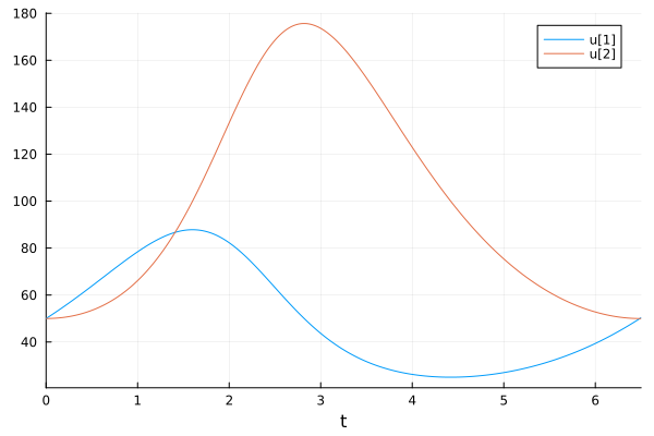
But if we want to draw a dependency then we will have to use slices . sol[1,:] and sol[2,:]. Which just reminds us of our aforementioned problem.
@btime plot(sol[1,:],sol[2,:])
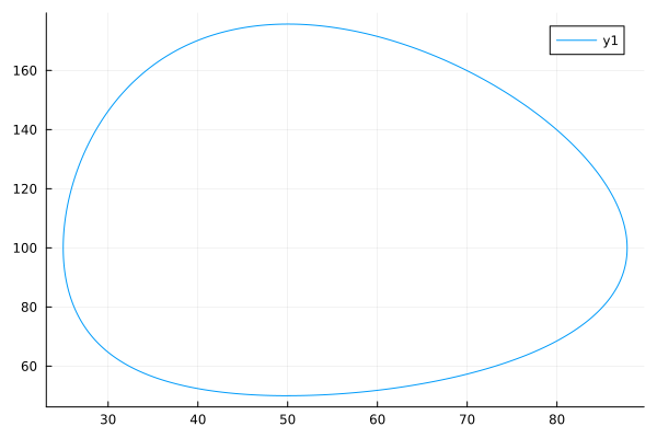
Which we can now solve using representations:
@btime @views plot(sol[1,:],sol[2,:])

Conclusions
After getting acquainted with the concept of representations, practical ways to improve the performance of functions that do not require any significant changes to the code were considered.