ControlSystems Plotting functions
|
All plotting requires the user to manually load the Plots.jl library, e.g., by calling |
#
ControlSystemsBase.bodeplot — Function
fig = bodeplot(sys, args...)
bodeplot(LTISystem[sys1, sys2...], args...; plotphase=true, balance = true, kwargs...)
Create a Bode plot of the LTISystem(s). A frequency vector w can be optionally provided. To change the Magnitude scale see setPlotScale. The default magnitude scale is "log10" (absolute scale).
-
If
hz=true, the plot x-axis will be displayed in Hertz, the input frequency vector is still treated as rad/s. -
balance: Callbalance_statespaceon the system before plotting.
kwargs is sent as argument to RecipesBase.plot.
#
ControlSystemsBase.gangoffourplot — Method
fig = gangoffourplot(P::LTISystem, C::LTISystem; minimal=true, plotphase=false, Ms_lines = [1.0, 1.25, 1.5], Mt_lines = [], sigma = true, kwargs...)Gang-of-Four plot.
sigma determines whether a sigmaplot is used instead of a bodeplot for MIMO S and T. kwargs are sent as argument to RecipesBase.plot.
#
ControlSystemsBase.marginplot — Function
fig = marginplot(sys::LTISystem [,w::AbstractVector];  balance=true, kwargs...)
marginplot(sys::Vector{LTISystem}, w::AbstractVector;  balance=true, kwargs...)
Plot all the amplitude and phase margins of the system(s) sys.
-
A frequency vector
wcan be optionally provided. -
balance: Callbalance_statespaceon the system before plotting.
kwargs is sent as argument to RecipesBase.plot.
#
ControlSystemsBase.nicholsplot — Function
fig = nicholsplot{T<:LTISystem}(systems::Vector{T}, w::AbstractVector; kwargs...)Create a Nichols plot of the LTISystem(s). A frequency vector w can be optionally provided.
Keyword arguments:
text = true
Gains = [12, 6, 3, 1, 0.5, -0.5, -1, -3, -6, -10, -20, -40, -60]
pInc = 30
sat = 0.4
val = 0.85
fontsize = 10
pInc determines the increment in degrees between phase lines.
sat ∈ [0,1] determines the saturation of the gain lines
val ∈ [0,1] determines the brightness of the gain lines
Additional keyword arguments are sent to the function plotting the systems and can be used to specify colors, line styles etc. using regular RecipesBase.jl syntax
This function is based on code subject to the two-clause BSD licence Copyright 2011 Will Robertson Copyright 2011 Philipp Allgeuer
#
ControlSystemsBase.nyquistplot — Function
fig = nyquistplot(sys;                Ms_circles=Float64[], Mt_circles=Float64[], unit_circle=false, hz=false, critical_point=-1, kwargs...)
nyquistplot(LTISystem[sys1, sys2...]; Ms_circles=Float64[], Mt_circles=Float64[], unit_circle=false, hz=false, critical_point=-1, kwargs...)
Create a Nyquist plot of the LTISystem(s). A frequency vector w can be optionally provided.
-
unit_circle: if the unit circle should be displayed. The Nyquist curve crosses the unit circle at the gain crossover frequency. -
Ms_circles: draw circles corresponding to given levels of sensitivity (circles around -1 with radii1/Ms).Ms_circlescan be supplied as a number or a vector of numbers. A design staying outside such a circle has a phase margin of at least2asin(1/(2Ms))rad and a gain margin of at leastMs/(Ms-1). -
Mt_circles: draw circles corresponding to given levels of complementary sensitivity.Mt_circlescan be supplied as a number or a vector of numbers. -
critical_point: point on real axis to mark as critical for encirclements -
If
hz=true, the hover information will be displayed in Hertz, the input frequency vector is still treated as rad/s. -
balance: Callbalance_statespaceon the system before plotting.
kwargs is sent as argument to plot.
#
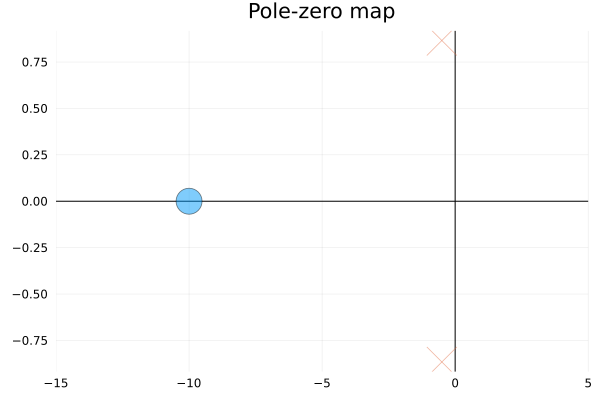
ControlSystemsBase.pzmap — Function
fig = pzmap(fig, system, args...; hz = false, kwargs...)Create a pole-zero map of the LTISystem(s) in figure fig, args and kwargs will be sent to the scatter plot command.
To customize the unit-circle drawn for discrete systems, modify the line attributes, e.g., linecolor=:red.
If hz is true, all poles and zeros are scaled by 1/2π.
#
ControlSystemsBase.rgaplot — Function
rgaplot(sys, args...; hz=false)
rgaplot(LTISystem[sys1, sys2...], args...; hz=false, balance=true)
Plot the relative-gain array entries of the LTISystem(s). A frequency vector w can be optionally provided.
-
If
hz=true, the plot x-axis will be displayed in Hertz, the input frequency vector is still treated as rad/s. -
balance: Callbalance_statespaceon the system before plotting.
kwargs is sent as argument to Plots.plot.
#
ControlSystemsBase.setPlotScale — Method
setPlotScale(str)Set the default scale of magnitude in bodeplot and sigmaplot. str should be either "dB" or "log10". The default scale if none is chosen is "log10".
#
ControlSystemsBase.sigmaplot — Function
sigmaplot(sys, args...; hz=false balance=true, extrema)
sigmaplot(LTISystem[sys1, sys2...], args...; hz=false, balance=true, extrema)
Plot the singular values of the frequency response of the LTISystem(s). A frequency vector w can be optionally provided.
-
If
hz=true, the plot x-axis will be displayed in Hertz, the input frequency vector is still treated as rad/s. -
balance: Callbalance_statespaceon the system before plotting. -
extrema: Only plot the largest and smallest singular values.
kwargs is sent as argument to Plots.plot.
Examples
Bode plot

tf1 = tf([1],[1,1])
tf2 = tf([1/5,2],[1,1,1])
sys = [tf1 tf2]
ws = exp10.(range(-2,stop=2,length=200))
bodeplot(sys, ws)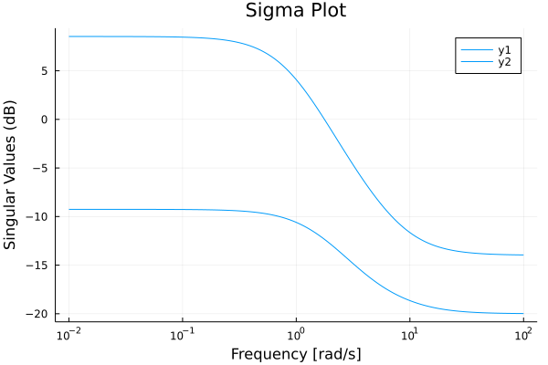
Margin

tf1 = tf([1],[1,1])
tf2 = tf([1/5,2],[1,1,1])
ws = exp10.(range(-2,stop=2,length=200))
marginplot([tf1, tf2], ws)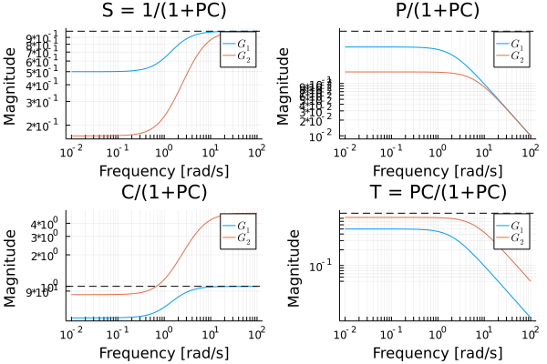
Nyquist plot

sys = ss([-1 2; 0 1], [1 0; 1 1], [1 0; 0 1], [0.1 0; 0 -0.2])
ws = exp10.(range(-2,stop=2,length=200))
nyquistplot(sys, ws, Ms_circles=1.2, Mt_circles=1.2)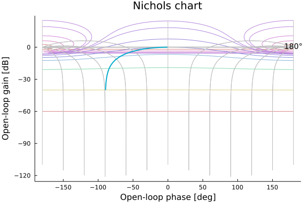
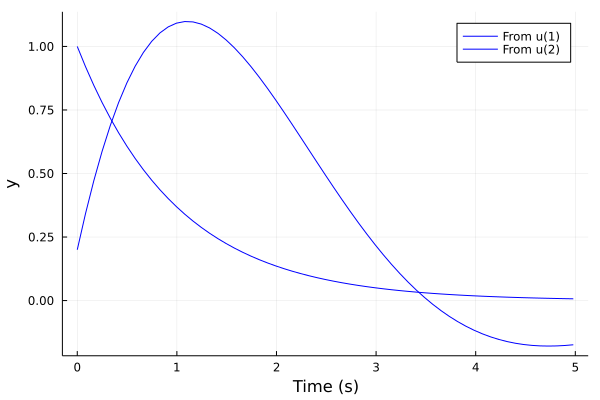
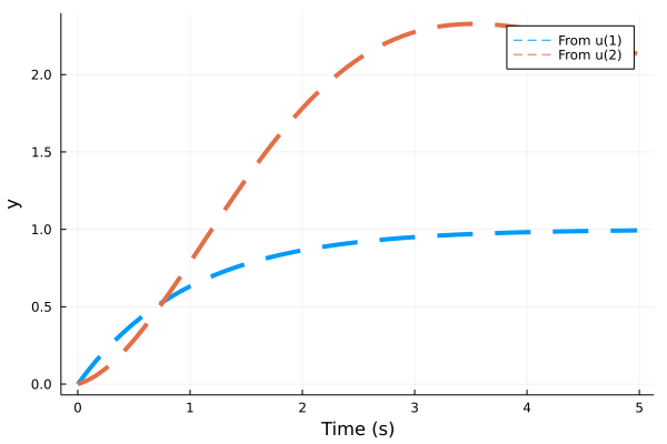
Lsim response plot

sys = ss([-1 2; 0 1], [1 0; 1 1], [1 0; 0 1], [0.1 0; 0 -0.2])
sysd = c2d(sys, 0.01)
L = lqr(sysd, [1 0; 0 1], [1 0; 0 1])
ts = 0:0.01:5
plot(lsim(sysd, (x,i)->-L*x, ts; x0=[1;2]), plotu=true)