EngeeRadars.TwoRayChannel

A two–beam propagation channel is the next step in complexity after a free-space channel and the simplest case of a multipath propagation medium.

The free space channel simulates a line-of-sight beam from point 1 to point 2.

In a two-beam channel, the medium is defined as a homogeneous, isotropic medium with a reflective flat boundary. The boundary is always set as .

There are no more than two rays propagating from point 1 to point 2. The first ray propagates along the same line-of-sight trajectory as in the channel of free space. The line-of-sight path is often referred to as a forward beam. The second ray is reflected from the boundary before hitting point 2. According to the law of reflection, the angle of reflection is equal to the angle of incidence. When simulating a short–range action, for example, in cellular communication systems or car radars, it can be assumed that the reflecting surface - the earth or the ocean surface – is flat.

System object EngeeRadars.TwoRayChannel simulates propagation time delay, phase shift, Doppler shift, and loss effects for both paths. For the reflected path, loss effects include reflection losses at the boundary.

The following figure shows two distribution paths. Based on the position of the source, , and receiver positions, you can calculate the angles of incidence for both paths, and . The angles of incidence are the angles of the location and azimuth of the incoming radiation relative to the local coordinate system. In this case, the local coordinate system coincides with the global coordinate system.

You can also calculate the propagation angles., and . In global coordinates, the reflection angle at the boundary coincides with the angles and . The reflection angle is important to know when you are using angle-dependent reflection loss data.

The total length of the path for the line-of-sight trajectory , which is equal to the geometric distance between the source and receiver, is shown in the figure.

The total length of the path for the reflected trajectory is . Value – this is the distance between the source and the receiver.

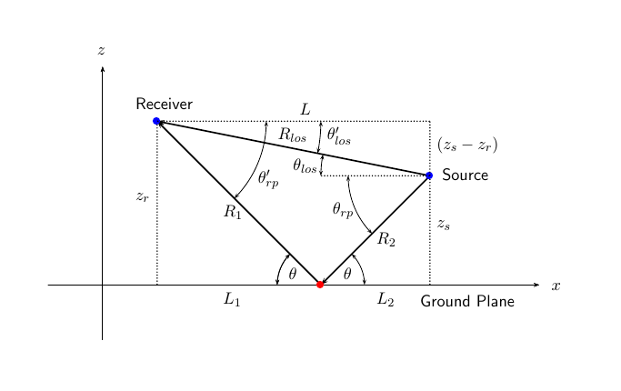
You can easily derive precise formulas for the path length and angles in terms of the distance to the ground and the height of objects in the global coordinate system.

Attenuation, or loss along the path in a two-beam channel, is the product of five components , where

Each component is specified in units of magnitude, not in dB.

Losses occur when the signal is reflected from the boundary. You can get a simple model of reflection losses from the earth by representing the electromagnetic field as a scalar field. This approach also works for acoustic and sonar systems.

Let – this is a scalar electromagnetic field of free space with an amplitude of at the control distance from the transmitter (for example, one meter). A field propagating in free space at a distance from the emitter it has the form

for the line-of-sight trajectory.

You can express what is reflected from the ground. - the field is like

where – the distance of the reflected path.

Value represents the losses associated with reflection from the ground plane. To specify , use the GroundReflectionCoefficient property. In the general case depends on the angle of incidence of the field. The total field at the destination is the sum of the fields of the line of sight and the reflected path.

For electromagnetic waves, a more complex but more realistic model uses a vector representation of a polarized field. You can decompose the incident electric field into two components. One component, , is parallel to the plane of incidence. Another component, , is perpendicular to the plane of incidence. The coefficients of reflection from the ground for these components are different and can be written in terms of ground permeability and angle of incidence.

where – the impedance of the medium. Since the magnetic permeability of the earth is almost the same as that of air or free space, the impedance ratio depends primarily on the ratio of electrical permeability.

where is the value – this is the relative permeability of the earth, set by the GroundRelativePermittivity property. Corner – this is the angle of incidence, and the angle – the angle of refraction at the boundary. You can define using Snell’s law of refraction.

After reflection, the total field is restored from the parallel and perpendicular components. Total attenuation in the ground plane, , is a combination of and .

When the starting point and destination point are stationary relative to each other, you can write the output of the Y object as . Value – this is the delay of the signal, and – losses on the way in free space. Delay set by . – this is either the distance of the propagation path in the line of sight, or the distance of the reflection path, and – the speed of propagation. Losses on the way:

where – the wavelength of the signal.

This model calculates the attenuation of signals propagating through atmospheric gases.

Electromagnetic signals are attenuated as they propagate through the atmosphere. This effect is mainly due to the resonant absorption lines of oxygen and water vapor, with nitrogen contributing less.

The model also includes a continuous absorption spectrum below 10 GHz.

The model calculates the specific attenuation (attenuation per kilometer) as a function of temperature, pressure, water vapor density, and signal frequency. The atmospheric gas model is valid for frequencies from 1-1000 GHz and is applicable to polarized and unpolarized fields.

The formula for the specific attenuation at each frequency:

Value It is an imaginary part of the complex atmospheric refraction and consists of a spectral line component and a continuous component.:

The spectral component consists of the sum of discrete spectral terms consisting of a localized function of the frequency band, multiplied by the strength of the spectral line, . For atmospheric oxygen, the strength of each spectral line is:

For atmospheric water vapor, the strength of each spectral line is:

this is the pressure of dry air, – partial pressure of water vapor, and – ambient temperature. The units of pressure measurement are hectopascals (gPa), and temperatures are degrees Kelvin. Partial pressure of water vapor, , is related to the density of water vapor, , as follows:

The total atmospheric pressure is + .

For each oxygen line depends on two parameters, and . Similarly, each water vapor line depends on two parameters, and . The ITU documentation at the end of this section contains tables of these parameters as functions of frequency.

Localized bandwidth functions they are complex frequency functions described in the ITU references given below. These functions depend on the empirical parameters of the model, which are also given in the references.

To calculate the total attenuation for narrowband signals on a path, the function multiplies the specific attenuation by the path length., . Then the total attenuation is .

You can apply the attenuation model to broadband signals. First, divide the broadband signal into frequency sub-bands and apply attenuation to each sub-band. Then sum up all the attenuated subband signals into a total attenuated signal.

This model calculates the attenuation of signals propagating through fog or clouds.

The weakening of fog and clouds is one and the same atmospheric phenomenon. The ITU model is used, _ Recommendation ITU-R P.840-6: Attenuation due to clouds and fog_. The model calculates the specific attenuation (attenuation per kilometer) of a signal as a function of liquid water density, signal frequency, and temperature. The model is applicable to polarized and unpolarized fields. The formula for the specific attenuation at each frequency is as follows

where – density of liquid water in gm/m3. Value It represents the specific attenuation coefficient and depends on the frequency. The cloud and fog attenuation model is valid for frequencies of 10-1000 GHz. The units of measurement of the specific attenuation coefficient are (dB/km)/(g/m3).

To calculate the total attenuation for narrowband signals on a path, the function multiplies the specific attenuation by the path length. . The total attenuation is .

You can apply the attenuation model to broadband signals. First, divide the broadband signal into frequency sub-bands and apply narrowband attenuation to each sub-band. Then sum up all the attenuated subband signals into a total attenuated signal.

This model calculates the attenuation of signals that propagate through regions with precipitation. Rain attenuation is the dominant attenuation mechanism and can vary from place to place and from year to year.

Electromagnetic signals are attenuated as they propagate through the precipitation area. Rain attenuation is calculated according to the ITU model for rain "_ITU-R Recommendation P.838-3: A specific attenuation model for rain for use in forecasting methods." The model calculates the specific attenuation (attenuation per kilometer) of a signal as a function of rain intensity, nominal signal frequency, polarization, and location angle. Specific attenuation, , is modeled as a power law depending on the rain velocity:

where – the speed of the rain. The units of measurement are mm/hour. Parameter and the exhibitor They depend on the frequency, the state of polarization, and the angle of the location on the signal path. The specific attenuation model is valid for frequencies from 1-1000 GHz.

To calculate the total attenuation for narrowband signals on the path, the function multiplies the specific attenuation by the effective propagation distance., . Then the total attenuation is .

The effective distance is the geometric distance, multiplied by the scale factor:

where – frequency. In the article "ITU-R Recommendation P.530-17 (12/2017): Propagation data and forecasting methods required for the design of ground-based line-of-sight systems_" contains a complete description of the attenuation calculation.

Rain rate, The one used in these calculations is the long–term statistical rain rate, . This is the rain rate, which is exceeded in 0.01% of cases. The calculation of the statistical precipitation norm is discussed in the ITU-R Recommendation P.837-7 (06/2017): Precipitation characteristics for propagation Modeling. This article also explains how to calculate the attenuation for other percentages of the 0.01% value.

You can apply the attenuation model to broadband signals. First, divide the broadband signal into frequency sub-bands and apply attenuation to each sub-band. Then sum up all the attenuated subband signals into a total attenuated signal.