Meshes
|
Страница в процессе перевода. |
Meshes can be constructed directly (e.g. CartesianGrid) or based on other constructs such as connectivity lists and topological structures (e.g. SimpleMesh).
Overview
#
Meshes.Mesh — Type
Mesh{M,CRS,TP}A mesh of geometries in a given manifold M with point coordinates specified in a coordinate reference system CRS. Unlike a general domain, a mesh has a well-defined topology TP.
#
Meshes.Grid — Type
Grid{M,CRS,Dim}A grid of geometries in a given manifold M with points coordinates specified in a coordinate reference system CRS, which is embedded in Dim dimensions.
#
Meshes.RegularGrid — Type
RegularGrid(dims, origin, spacing)A regular grid with dimensions dims, lower left corner at origin and cell spacing spacing. The three arguments must have the same length.
RegularGrid(dims, origin, spacing, offset)
A regular grid with dimensions dims, with lower left corner of element offset at origin and cell spacing spacing.
RegularGrid(start, finish, dims=dims)
Alternatively, construct a regular grid from a start point to a finish with dimensions dims.
RegularGrid(start, finish, spacing)
Alternatively, construct a regular grid from a start point to a finish point using a given spacing.
Examples
RegularGrid((10, 20), Point(LatLon(30.0°, 60.0°)), (1.0, 1.0)) # add coordinate units to spacing
RegularGrid((10, 20), Point(Polar(0.0cm, 0.0rad)), (10.0mm, 1.0rad)) # convert spacing units to coordinate units
RegularGrid((10, 20), Point(Mercator(0.0, 0.0)), (1.5, 1.5))
RegularGrid((10, 20, 30), Point(Cylindrical(0.0, 0.0, 0.0)), (3.0, 2.0, 1.0))
See also CartesianGrid.
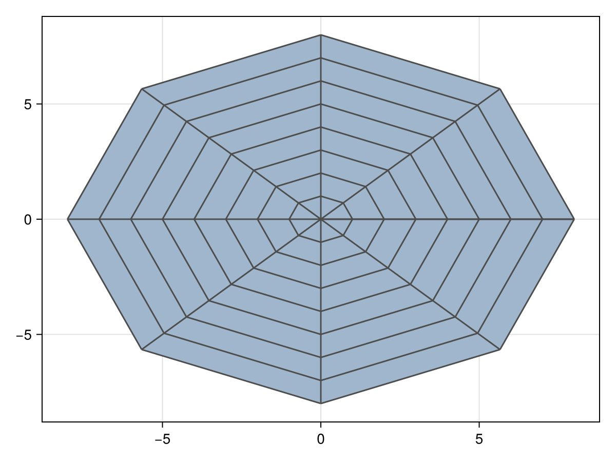
# 2D regular grid
grid = RegularGrid((8, 8), Point(Polar(0, 0)), (1, π/4))

viz(grid, showsegments = true)
#
Meshes.CartesianGrid — Type
CartesianGrid(dims, origin, spacing)A Cartesian grid with dimensions dims, lower left corner at origin and cell spacing spacing. The three arguments must have the same length.
CartesianGrid(dims, origin, spacing, offset)
A Cartesian grid with dimensions dims, with lower left corner of element offset at origin and cell spacing spacing.
CartesianGrid(start, finish, dims=dims)
Alternatively, construct a Cartesian grid from a start point (lower left) to a finish point (upper right).
CartesianGrid(start, finish, spacing)
Alternatively, construct a Cartesian grid from a start point to a finish point using a given spacing.
CartesianGrid(dims)
CartesianGrid(dim1, dim2, ...)
Finally, a Cartesian grid can be constructed by only passing the dimensions dims as a tuple, or by passing each dimension dim1, dim2, … separately. In this case, the origin and spacing default to (0,0,…) and (1,1,…).
CartesianGrid is an alias to RegularGrid with Cartesian CRS.
Examples
Create a 3D grid with 100x100x50 hexahedrons:
julia> CartesianGrid(100, 100, 50)Create a 2D grid with 100 x 100 quadrangles and origin at (10.0, 20.0):
julia> CartesianGrid((100, 100), (10.0, 20.0), (1.0, 1.0))Create a 1D grid from -1 to 1 with 100 segments:
julia> CartesianGrid((-1.0,), (1.0,), dims=(100,))See also RegularGrid.
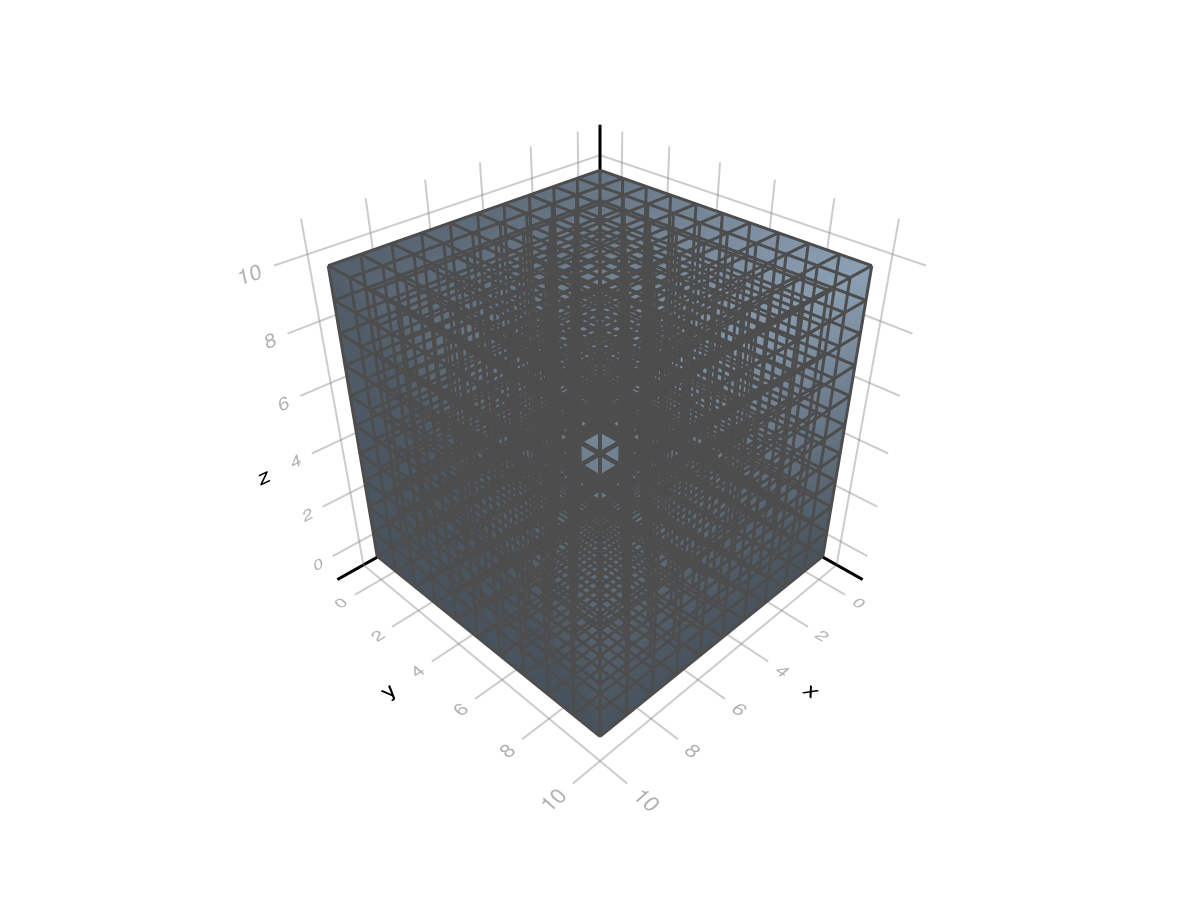
# 3D Cartesian grid
grid = CartesianGrid(10, 10, 10)

viz(grid, showsegments = true)
#
Meshes.RectilinearGrid — Type
RectilinearGrid(x, y, z, ...)
RectilinearGrid{M,C}(x, y, z, ...)
A rectilinear grid with vertices at sorted coordinates x, y, z, …, manifold M (default to 𝔼) and CRS type C (default to Cartesian).
Examples
Create a 2D rectilinear grid with regular spacing in x dimension and irregular spacing in y dimension:
julia> x = 0.0:0.2:1.0
julia> y = [0.0, 0.1, 0.3, 0.7, 0.9, 1.0]
julia> RectilinearGrid(x, y)
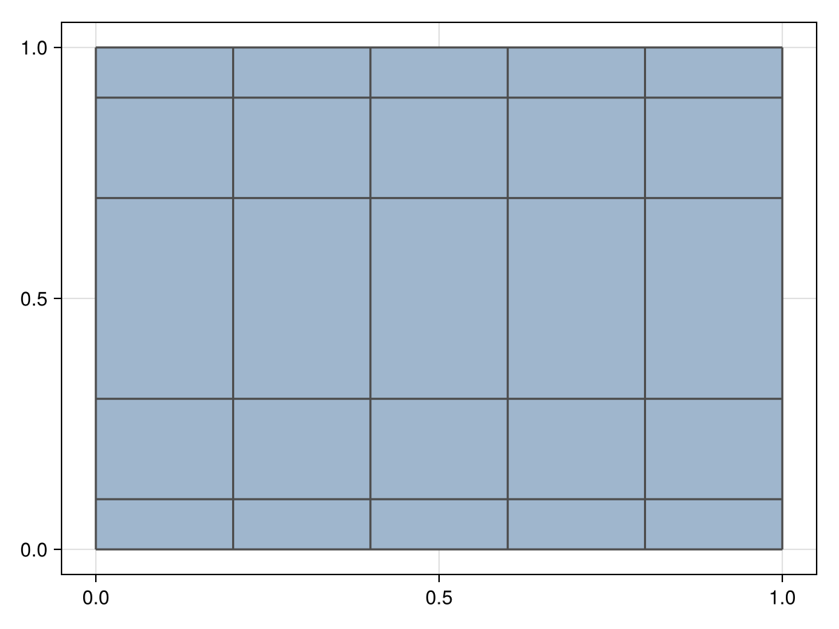
# 2D rectilinear grid
x = 0.0:0.2:1.0
y = [0.0, 0.1, 0.3, 0.7, 0.9, 1.0]
grid = RectilinearGrid(x, y)
viz(grid, showsegments = true)
#
Meshes.StructuredGrid — Type
StructuredGrid(X, Y, Z, ...)
StructuredGrid{M,C}(X, Y, Z, ...)
A structured grid with vertices at sorted coordinates X, Y, Z, …, manifold M (default to 𝔼) and CRS type C (default to Cartesian).
Examples
Create a 2D structured grid with regular spacing in x dimension and irregular spacing in y dimension:
julia> X = repeat(0.0:0.2:1.0, 1, 6)
julia> Y = repeat([0.0, 0.1, 0.3, 0.7, 0.9, 1.0]', 6, 1)
julia> StructuredGrid(X, Y)
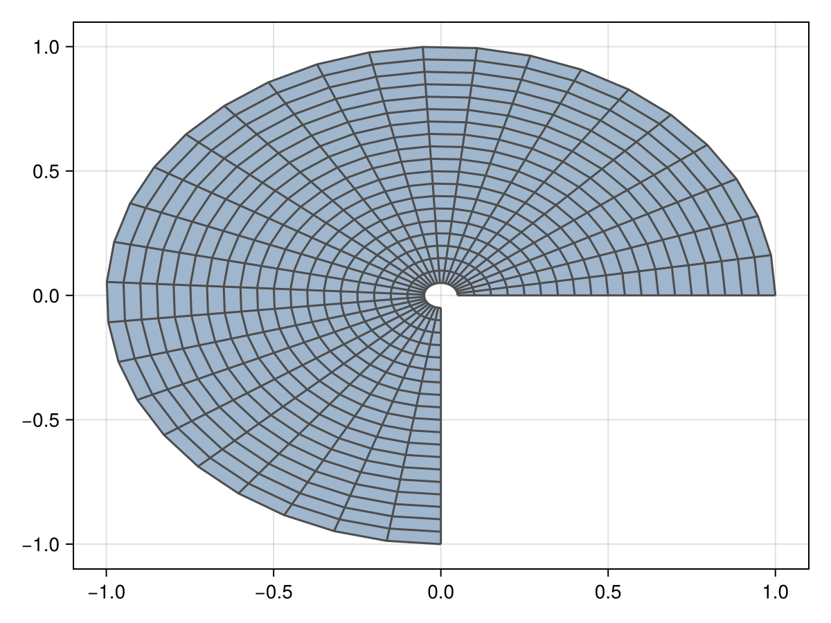
# 2D structured grid
X = [i/20 * cos(3π/2 * (j-1) / (30-1)) for i in 1:20, j in 1:30]
Y = [i/20 * sin(3π/2 * (j-1) / (30-1)) for i in 1:20, j in 1:30]
grid = StructuredGrid(X, Y)
viz(grid, showsegments = true)
#
Meshes.SimpleMesh — Type
SimpleMesh(vertices, topology)A simple mesh with vertices and topology.
SimpleMesh(vertices, connectivities; relations=false)
Alternatively, construct a simple mesh with vertices and connectivities. The option relations can be used to build topological relations assuming that the connectivities represent the elements of the mesh.
Examples
julia> points = [(0.0, 0.0),(1.0, 0.0), (1.0, 1.0)]
julia> connec = [connect((1,2,3))]
julia> mesh   = SimpleMesh(points, connec)
See also Topology, GridTopology, HalfEdgeTopology, SimpleTopology.
Notes
-
The option
relations=truechanges the underlying topology of the mesh to aHalfEdgeTopologyinstead of aSimpleTopology.
# global vector of 2D points
points = [(0,0),(1,0),(0,1),(1,1),(0.25,0.5),(0.75,0.5)]

# connect the points into N-gon
connec = connect.([(1,2,6,5),(2,4,6),(4,3,5,6),(3,1,5)], Ngon)

# 2D mesh made of N-gon elements
mesh = SimpleMesh(points, connec)

viz(mesh, showsegments = true)
Connectivities
#
Meshes.connect — Function
connect(indices, [PL])The type PL can be a Ngon in which case the length of the indices is used to identify the actual polytope type.
Finally, the type PL can be ommitted. In this case, the indices are assumed to be connected as a Ngon or as a Segment.
Examples
Connect indices into a Triangle:
connect((1,2,3), Triangle)Connect indices into N-gons, a Triangle and a Quadrangle:
connect.([(1,2,3), (2,3,4,5)], Ngon)Connect indices into N-gon or segment:
connect((1,2)) # Segment
connect((1,2,3)) # Triangle
connect((1,2,3,4)) # Quadrangle
#
Meshes.materialize — Function
materialize(connec, points)Materialize a face using the connec list and a global vector of points.
Topology
#
Meshes.Topology — Type
TopologyA data structure for constructing topological relations in a Mesh.
References
-
Floriani, L. & Hui, A. 2007. Shape representations based on simplicial and cell complexes
#
Meshes.GridTopology — Type
GridTopology(dims, [periodic])A data structure for grid topologies with dims elements. Optionally, specify which dimensions are periodic. Default to aperiodic dimensions.
Examples
julia> GridTopology((10,20)) # 10x20 elements in a grid
julia> GridTopology((10,20), (true,false)) # cylinder topology
#
Meshes.HalfEdgeTopology — Type
HalfEdgeTopology(elements; sort=true)
HalfEdgeTopology(halfedges)
A data structure for orientable 2-manifolds based on half-edges constructed from a vector of connectivity elements or from a vector of pairs of halfedges.
The option sort can be used to sort the elements in adjacent-first order in case of inconsistent orientation (i.e. mix of clockwise and counter-clockwise).
Examples
Construct half-edge topology from a list of top-faces:
elements = connect.([(1,2,3),(3,2,4,5)])
topology = HalfEdgeTopology(elements)
See also Topology.
References
-
Kettner, L. (1999). Using generic programming for designing a data structure for polyhedral surfaces
Notes
-
Two types of half-edges exist (Kettner 1999). This implementation is the most common type that splits the incident elements.
-
A vector of
halfedgestogether with a dictionary ofhalf4elemand a dictionary ofhalf4vertcan be used to retrieve topolological relations in optimal time. In this case,half4vert[i]returns the index of the half-edge inhalfedgeswith head equal toi. Similarly,half4elem[i]returns the index of a half-edge inhalfedgesthat is in the elementi. Additionally, a dictionaryedge4pairreturns the index of the edge (i.e. two halves) for a given pair of vertices. -
If the
elementsof the mesh already have consistent orientation, then thesortoption can be disabled for maximum performance.
#
Meshes.SimpleTopology — Type
SimpleTopology(connectivities)A data structure that stores all connectivities of a mesh.
Notes
This data structure is sometimes referred to as the "soup of geometries". It does not support topological relations and is therefore incompatible with algorithms that rely on neighborhood search. It is still useful for mesh visualization and IO operations.
Relations
#
Meshes.TopologicalRelation — Type
TopologicalRelationAn object implementing this trait is a functor that can be evaluated at an integer index representing the face.
Examples
# create boundary relation mapping
# 2-faces to 0-faces (i.e. vertices)
∂ = Boundary{2,0}(topology)

# list of vertices for first face
∂(1)
References
-
Floriani, L. & Hui, A. 2007. Shape representations based on simplicial and cell complexes
#
Meshes.Boundary — Type
Boundary{P,Q}(topology)The boundary relation from rank P to smaller rank Q for a given topology.
#
Meshes.Coboundary — Type
Coboundary{P,Q}(topology)The co-boundary relation from rank P to greater rank Q for a given topology.
#
Meshes.Adjacency — Type
Adjacency{P}(topology)The adjacency relation of rank P for a given topology.
Consider the following examples with the Boundary and Coboundary relations defined for the HalfEdgeTopology:
# global vector of 2D points
points = [(0,0),(1,0),(0,1),(1,1),(0.25,0.5),(0.75,0.5)]

# connect the points into N-gon
connec = connect.([(1,2,6,5),(2,4,6),(4,3,5,6),(3,1,5)], Ngon)

# 2D mesh made of N-gon elements
mesh = SimpleMesh(points, connec)
4 SimpleMesh
6 vertices
├─ Point(x: 0.0 m, y: 0.0 m)
├─ Point(x: 1.0 m, y: 0.0 m)
├─ Point(x: 0.0 m, y: 1.0 m)
├─ Point(x: 1.0 m, y: 1.0 m)
├─ Point(x: 0.25 m, y: 0.5 m)
└─ Point(x: 0.75 m, y: 0.5 m)
4 elements
├─ Quadrangle(1, 2, 6, 5)
├─ Triangle(2, 4, 6)
├─ Quadrangle(4, 3, 5, 6)
└─ Triangle(3, 1, 5)# convert topology to half-edge topology
topo = convert(HalfEdgeTopology, topology(mesh))
# boundary relation from faces (dim=2) to edges (dim=1)
∂₂₁ = Boundary{2,1}(topo)
# show boundary of first n-gon
∂₂₁(1)(1, 3, 5, 6)# co-boundary relation from edges (dim=1) to faces(dim=2)
𝒞₁₂ = Coboundary{1,2}(topo)
# show n-gons that share edge 3
𝒞₁₂(3)(2, 1)Matrices
Based on topological relations, we can extract matrices that are widely used in applications such as laplacematrix, and adjacencymatrix.
Laplace
#
Meshes.laplacematrix — Function
laplacematrix(mesh; kind=nothing)The Laplace-Beltrami (a.k.a. Laplacian) matrix of the mesh. Optionally, specify the kind of discretization.
Available discretizations
-
:uniform-Lᵢⱼ = 1 / |𝒜(i)|, ∀j ∈ 𝒜(i) -
:cotangent-Lᵢⱼ = cot(αᵢⱼ) + cot(βᵢⱼ), ∀j ∈ 𝒜(i)
where 𝒜(i) is the adjacency relation at vertex i.
References
-
Botsch et al. 2010. Polygon Mesh Processing.
-
Pinkall, U. & Polthier, K. 1993. Computing discrete minimal surfaces and their conjugates.
grid = CartesianGrid(10, 10)

laplacematrix(grid, kind = :uniform)
121×121 SparseArrays.SparseMatrixCSC{Float64, Int64} with 561 stored entries:
⎡⠻⣦⡀⠈⠲⣀⠀⠀⠀⠀⠀⠀⠀⠀⠀⠀⠀⠀⠀⠀⠀⠀⠀⠀⠀⠀⠀⠀⠀⠀⠀⠀⠀⠀⠀⠀⠀⠀⠀⠀⎤
⎢⡀⠈⠻⣦⡀⠈⠲⡀⠀⠀⠀⠀⠀⠀⠀⠀⠀⠀⠀⠀⠀⠀⠀⠀⠀⠀⠀⠀⠀⠀⠀⠀⠀⠀⠀⠀⠀⠀⠀⠀⎥
⎢⠘⢢⡀⠈⠻⣦⡀⠈⠢⡀⠀⠀⠀⠀⠀⠀⠀⠀⠀⠀⠀⠀⠀⠀⠀⠀⠀⠀⠀⠀⠀⠀⠀⠀⠀⠀⠀⠀⠀⠀⎥
⎢⠀⠀⠘⠢⡀⠈⠻⣦⡀⠈⠢⡄⠀⠀⠀⠀⠀⠀⠀⠀⠀⠀⠀⠀⠀⠀⠀⠀⠀⠀⠀⠀⠀⠀⠀⠀⠀⠀⠀⠀⎥
⎢⠀⠀⠀⠀⠈⠢⡀⠈⠻⣦⡀⠈⠣⡄⠀⠀⠀⠀⠀⠀⠀⠀⠀⠀⠀⠀⠀⠀⠀⠀⠀⠀⠀⠀⠀⠀⠀⠀⠀⠀⎥
⎢⠀⠀⠀⠀⠀⠀⠈⠦⡀⠈⠛⣤⡀⠈⠣⡄⠀⠀⠀⠀⠀⠀⠀⠀⠀⠀⠀⠀⠀⠀⠀⠀⠀⠀⠀⠀⠀⠀⠀⠀⎥
⎢⠀⠀⠀⠀⠀⠀⠀⠀⠉⠦⡀⠈⠻⣦⡀⠈⠣⡄⠀⠀⠀⠀⠀⠀⠀⠀⠀⠀⠀⠀⠀⠀⠀⠀⠀⠀⠀⠀⠀⠀⎥
⎢⠀⠀⠀⠀⠀⠀⠀⠀⠀⠀⠉⠦⡀⠈⠱⣦⡀⠈⠣⡄⠀⠀⠀⠀⠀⠀⠀⠀⠀⠀⠀⠀⠀⠀⠀⠀⠀⠀⠀⠀⎥
⎢⠀⠀⠀⠀⠀⠀⠀⠀⠀⠀⠀⠀⠉⠦⡀⠈⠻⣦⡀⠈⠢⡀⠀⠀⠀⠀⠀⠀⠀⠀⠀⠀⠀⠀⠀⠀⠀⠀⠀⠀⎥
⎢⠀⠀⠀⠀⠀⠀⠀⠀⠀⠀⠀⠀⠀⠀⠉⠦⡀⠈⠻⣦⡀⠈⠢⣀⠀⠀⠀⠀⠀⠀⠀⠀⠀⠀⠀⠀⠀⠀⠀⠀⎥
⎢⠀⠀⠀⠀⠀⠀⠀⠀⠀⠀⠀⠀⠀⠀⠀⠀⠈⠢⡀⠈⠻⣦⡀⠈⠲⣀⠀⠀⠀⠀⠀⠀⠀⠀⠀⠀⠀⠀⠀⠀⎥
⎢⠀⠀⠀⠀⠀⠀⠀⠀⠀⠀⠀⠀⠀⠀⠀⠀⠀⠀⠈⢢⡀⠈⠻⣦⡀⠈⠲⣀⠀⠀⠀⠀⠀⠀⠀⠀⠀⠀⠀⠀⎥
⎢⠀⠀⠀⠀⠀⠀⠀⠀⠀⠀⠀⠀⠀⠀⠀⠀⠀⠀⠀⠀⠘⢢⡀⠈⠻⢆⡀⠈⠲⣀⠀⠀⠀⠀⠀⠀⠀⠀⠀⠀⎥
⎢⠀⠀⠀⠀⠀⠀⠀⠀⠀⠀⠀⠀⠀⠀⠀⠀⠀⠀⠀⠀⠀⠀⠘⢢⡀⠈⠻⣦⡀⠈⠲⣀⠀⠀⠀⠀⠀⠀⠀⠀⎥
⎢⠀⠀⠀⠀⠀⠀⠀⠀⠀⠀⠀⠀⠀⠀⠀⠀⠀⠀⠀⠀⠀⠀⠀⠀⠘⢢⡀⠈⠛⣤⡀⠈⠲⡀⠀⠀⠀⠀⠀⠀⎥
⎢⠀⠀⠀⠀⠀⠀⠀⠀⠀⠀⠀⠀⠀⠀⠀⠀⠀⠀⠀⠀⠀⠀⠀⠀⠀⠀⠘⢢⡀⠈⠻⣦⡀⠈⠢⡀⠀⠀⠀⠀⎥
⎢⠀⠀⠀⠀⠀⠀⠀⠀⠀⠀⠀⠀⠀⠀⠀⠀⠀⠀⠀⠀⠀⠀⠀⠀⠀⠀⠀⠀⠘⠢⡀⠈⠻⣦⡀⠈⠢⡄⠀⠀⎥
⎢⠀⠀⠀⠀⠀⠀⠀⠀⠀⠀⠀⠀⠀⠀⠀⠀⠀⠀⠀⠀⠀⠀⠀⠀⠀⠀⠀⠀⠀⠀⠈⠢⡀⠈⠻⣦⡀⠈⠣⡄⎥
⎢⠀⠀⠀⠀⠀⠀⠀⠀⠀⠀⠀⠀⠀⠀⠀⠀⠀⠀⠀⠀⠀⠀⠀⠀⠀⠀⠀⠀⠀⠀⠀⠀⠈⠦⡀⠈⠻⣦⡀⠈⎥
⎣⠀⠀⠀⠀⠀⠀⠀⠀⠀⠀⠀⠀⠀⠀⠀⠀⠀⠀⠀⠀⠀⠀⠀⠀⠀⠀⠀⠀⠀⠀⠀⠀⠀⠀⠉⠦⡀⠈⠻⣦⎦points = [(0, 0), (1, 0), (0, 1), (1, 1), (0.5, 0.5)]
connec = connect.([(1, 2, 5), (2, 4, 5), (4, 3, 5), (3, 1, 5)])
mesh = SimpleMesh(points, connec)
laplacematrix(mesh, kind = :cotangent)5×5 SparseArrays.SparseMatrixCSC{Float64, Int64} with 21 stored entries:
-0.0 -1.0 -1.0 ⋅ 2.0
-1.0 -0.0 ⋅ -1.0 2.0
-1.0 ⋅ -0.0 -1.0 2.0
⋅ -1.0 -1.0 -0.0 2.0
2.0 2.0 2.0 2.0 -8.0Measure
#
Meshes.measurematrix — Function
measurematrix(mesh)The measure (or "mass") matrix of the mesh, i.e. a diagonal matrix with entries Mᵢᵢ = 2Aᵢ where Aᵢ is (one-third of) the sum of the areas of triangles sharing vertex i.
The discrete cotangent Laplace-Beltrami operator can be written as Δ = M⁻¹L. When solving systems of the form Δu = f, it is useful to write Lu = Mf and exploit the symmetry of L.
grid = CartesianGrid(10, 10)

measurematrix(grid)
121×121 LinearAlgebra.Diagonal{Quantity{Float64, 𝐋^2, Unitful.FreeUnits{(m^2,), 𝐋^2, nothing}}, Vector{Quantity{Float64, 𝐋^2, Unitful.FreeUnits{(m^2,), 𝐋^2, nothing}}}}:
0.666667 m^2 ⋅ ⋅ … ⋅ ⋅
⋅ 1.33333 m^2 ⋅ ⋅ ⋅
⋅ ⋅ 1.33333 m^2 ⋅ ⋅
⋅ ⋅ ⋅ ⋅ ⋅
⋅ ⋅ ⋅ ⋅ ⋅
⋅ ⋅ ⋅ … ⋅ ⋅
⋅ ⋅ ⋅ ⋅ ⋅
⋅ ⋅ ⋅ ⋅ ⋅
⋅ ⋅ ⋅ ⋅ ⋅
⋅ ⋅ ⋅ ⋅ ⋅
⋮ ⋱ ⋮
⋅ ⋅ ⋅ ⋅ ⋅
⋅ ⋅ ⋅ ⋅ ⋅
⋅ ⋅ ⋅ ⋅ ⋅
⋅ ⋅ ⋅ … ⋅ ⋅
⋅ ⋅ ⋅ ⋅ ⋅
⋅ ⋅ ⋅ ⋅ ⋅
⋅ ⋅ ⋅ ⋅ ⋅
⋅ ⋅ ⋅ 1.33333 m^2 ⋅
⋅ ⋅ ⋅ … ⋅ 0.666667 m^2points = [(0, 0), (1, 0), (0, 1), (1, 1), (0.5, 0.5)]
connec = connect.([(1, 2, 5), (2, 4, 5), (4, 3, 5), (3, 1, 5)])
mesh = SimpleMesh(points, connec)
measurematrix(mesh)5×5 LinearAlgebra.Diagonal{Quantity{Float64, 𝐋^2, Unitful.FreeUnits{(m^2,), 𝐋^2, nothing}}, Vector{Quantity{Float64, 𝐋^2, Unitful.FreeUnits{(m^2,), 𝐋^2, nothing}}}}:
0.333333 m^2 ⋅ ⋅ ⋅ ⋅
⋅ 0.333333 m^2 ⋅ ⋅ ⋅
⋅ ⋅ 0.333333 m^2 ⋅ ⋅
⋅ ⋅ ⋅ 0.333333 m^2 ⋅
⋅ ⋅ ⋅ ⋅ 0.666667 m^2Adjacency
#
Meshes.adjacencymatrix — Function
adjacencymatrix(mesh; rank=paramdim(mesh))The adjacency matrix of the mesh using the adjacency relation of given rank for the underlying topology.
grid = CartesianGrid(10, 10)

adjacencymatrix(grid)
100×100 SparseArrays.SparseMatrixCSC{Int64, Int64} with 360 stored entries:
⎡⠪⡦⡀⠀⠑⢄⠀⠀⠀⠀⠀⠀⠀⠀⠀⠀⠀⠀⠀⠀⠀⠀⠀⠀⠀⠀⠀⠀⠀⠀⠀⠀⠀⠀⠀⠀⠀⠀⠀⠀⎤
⎢⠀⠈⠪⡦⠀⠀⠑⢄⠀⠀⠀⠀⠀⠀⠀⠀⠀⠀⠀⠀⠀⠀⠀⠀⠀⠀⠀⠀⠀⠀⠀⠀⠀⠀⠀⠀⠀⠀⠀⠀⎥
⎢⠑⢄⠀⠀⠪⡦⡀⠀⠑⢄⠀⠀⠀⠀⠀⠀⠀⠀⠀⠀⠀⠀⠀⠀⠀⠀⠀⠀⠀⠀⠀⠀⠀⠀⠀⠀⠀⠀⠀⠀⎥
⎢⠀⠀⠑⢄⠀⠈⠪⡦⠀⠀⠑⢄⠀⠀⠀⠀⠀⠀⠀⠀⠀⠀⠀⠀⠀⠀⠀⠀⠀⠀⠀⠀⠀⠀⠀⠀⠀⠀⠀⠀⎥
⎢⠀⠀⠀⠀⠑⢄⠀⠀⠪⡦⡀⠀⠑⢄⠀⠀⠀⠀⠀⠀⠀⠀⠀⠀⠀⠀⠀⠀⠀⠀⠀⠀⠀⠀⠀⠀⠀⠀⠀⠀⎥
⎢⠀⠀⠀⠀⠀⠀⠑⢄⠀⠈⠪⡦⠀⠀⠑⢄⠀⠀⠀⠀⠀⠀⠀⠀⠀⠀⠀⠀⠀⠀⠀⠀⠀⠀⠀⠀⠀⠀⠀⠀⎥
⎢⠀⠀⠀⠀⠀⠀⠀⠀⠑⢄⠀⠀⠪⡦⡀⠀⠑⢄⠀⠀⠀⠀⠀⠀⠀⠀⠀⠀⠀⠀⠀⠀⠀⠀⠀⠀⠀⠀⠀⠀⎥
⎢⠀⠀⠀⠀⠀⠀⠀⠀⠀⠀⠑⢄⠀⠈⠪⡦⠀⠀⠑⢄⠀⠀⠀⠀⠀⠀⠀⠀⠀⠀⠀⠀⠀⠀⠀⠀⠀⠀⠀⠀⎥
⎢⠀⠀⠀⠀⠀⠀⠀⠀⠀⠀⠀⠀⠑⢄⠀⠀⠪⡦⡀⠀⠱⢄⠀⠀⠀⠀⠀⠀⠀⠀⠀⠀⠀⠀⠀⠀⠀⠀⠀⠀⎥
⎢⠀⠀⠀⠀⠀⠀⠀⠀⠀⠀⠀⠀⠀⠀⠑⢄⠀⠈⠪⡦⠀⠀⠱⢄⠀⠀⠀⠀⠀⠀⠀⠀⠀⠀⠀⠀⠀⠀⠀⠀⎥
⎢⠀⠀⠀⠀⠀⠀⠀⠀⠀⠀⠀⠀⠀⠀⠀⠀⠑⢆⠀⠀⠺⡢⡀⠀⠑⢄⠀⠀⠀⠀⠀⠀⠀⠀⠀⠀⠀⠀⠀⠀⎥
⎢⠀⠀⠀⠀⠀⠀⠀⠀⠀⠀⠀⠀⠀⠀⠀⠀⠀⠀⠑⢆⠀⠈⠺⡢⠀⠀⠑⢄⠀⠀⠀⠀⠀⠀⠀⠀⠀⠀⠀⠀⎥
⎢⠀⠀⠀⠀⠀⠀⠀⠀⠀⠀⠀⠀⠀⠀⠀⠀⠀⠀⠀⠀⠑⢄⠀⠀⠺⡢⡀⠀⠑⢄⠀⠀⠀⠀⠀⠀⠀⠀⠀⠀⎥
⎢⠀⠀⠀⠀⠀⠀⠀⠀⠀⠀⠀⠀⠀⠀⠀⠀⠀⠀⠀⠀⠀⠀⠑⢄⠀⠈⠺⡢⠀⠀⠑⢄⠀⠀⠀⠀⠀⠀⠀⠀⎥
⎢⠀⠀⠀⠀⠀⠀⠀⠀⠀⠀⠀⠀⠀⠀⠀⠀⠀⠀⠀⠀⠀⠀⠀⠀⠑⢄⠀⠀⠺⡢⡀⠀⠑⢄⠀⠀⠀⠀⠀⠀⎥
⎢⠀⠀⠀⠀⠀⠀⠀⠀⠀⠀⠀⠀⠀⠀⠀⠀⠀⠀⠀⠀⠀⠀⠀⠀⠀⠀⠑⢄⠀⠈⠺⡢⠀⠀⠑⢄⠀⠀⠀⠀⎥
⎢⠀⠀⠀⠀⠀⠀⠀⠀⠀⠀⠀⠀⠀⠀⠀⠀⠀⠀⠀⠀⠀⠀⠀⠀⠀⠀⠀⠀⠑⢄⠀⠀⠺⡢⡀⠀⠑⢄⠀⠀⎥
⎢⠀⠀⠀⠀⠀⠀⠀⠀⠀⠀⠀⠀⠀⠀⠀⠀⠀⠀⠀⠀⠀⠀⠀⠀⠀⠀⠀⠀⠀⠀⠑⢄⠀⠈⠺⡢⠀⠀⠑⢄⎥
⎢⠀⠀⠀⠀⠀⠀⠀⠀⠀⠀⠀⠀⠀⠀⠀⠀⠀⠀⠀⠀⠀⠀⠀⠀⠀⠀⠀⠀⠀⠀⠀⠀⠑⢄⠀⠀⠺⡢⡀⠀⎥
⎣⠀⠀⠀⠀⠀⠀⠀⠀⠀⠀⠀⠀⠀⠀⠀⠀⠀⠀⠀⠀⠀⠀⠀⠀⠀⠀⠀⠀⠀⠀⠀⠀⠀⠀⠑⢄⠀⠈⠺⡢⎦adjacencymatrix(grid, rank = 0)121×121 SparseArrays.SparseMatrixCSC{Int64, Int64} with 440 stored entries:
⎡⠺⣢⡀⠈⠲⣀⠀⠀⠀⠀⠀⠀⠀⠀⠀⠀⠀⠀⠀⠀⠀⠀⠀⠀⠀⠀⠀⠀⠀⠀⠀⠀⠀⠀⠀⠀⠀⠀⠀⠀⎤
⎢⡀⠈⠺⡢⡀⠈⠲⡀⠀⠀⠀⠀⠀⠀⠀⠀⠀⠀⠀⠀⠀⠀⠀⠀⠀⠀⠀⠀⠀⠀⠀⠀⠀⠀⠀⠀⠀⠀⠀⠀⎥
⎢⠘⢢⡀⠈⠺⣢⡀⠈⠢⡀⠀⠀⠀⠀⠀⠀⠀⠀⠀⠀⠀⠀⠀⠀⠀⠀⠀⠀⠀⠀⠀⠀⠀⠀⠀⠀⠀⠀⠀⠀⎥
⎢⠀⠀⠘⠢⡀⠈⠺⡢⡀⠈⠢⡄⠀⠀⠀⠀⠀⠀⠀⠀⠀⠀⠀⠀⠀⠀⠀⠀⠀⠀⠀⠀⠀⠀⠀⠀⠀⠀⠀⠀⎥
⎢⠀⠀⠀⠀⠈⠢⡀⠈⠫⡦⡀⠈⠣⡄⠀⠀⠀⠀⠀⠀⠀⠀⠀⠀⠀⠀⠀⠀⠀⠀⠀⠀⠀⠀⠀⠀⠀⠀⠀⠀⎥
⎢⠀⠀⠀⠀⠀⠀⠈⠦⡀⠈⠋⡤⡀⠈⠣⡄⠀⠀⠀⠀⠀⠀⠀⠀⠀⠀⠀⠀⠀⠀⠀⠀⠀⠀⠀⠀⠀⠀⠀⠀⎥
⎢⠀⠀⠀⠀⠀⠀⠀⠀⠉⠦⡀⠈⠫⡦⡀⠈⠣⡄⠀⠀⠀⠀⠀⠀⠀⠀⠀⠀⠀⠀⠀⠀⠀⠀⠀⠀⠀⠀⠀⠀⎥
⎢⠀⠀⠀⠀⠀⠀⠀⠀⠀⠀⠉⠦⡀⠈⠡⡦⡀⠈⠣⡄⠀⠀⠀⠀⠀⠀⠀⠀⠀⠀⠀⠀⠀⠀⠀⠀⠀⠀⠀⠀⎥
⎢⠀⠀⠀⠀⠀⠀⠀⠀⠀⠀⠀⠀⠉⠦⡀⠈⠫⡦⡀⠈⠢⡀⠀⠀⠀⠀⠀⠀⠀⠀⠀⠀⠀⠀⠀⠀⠀⠀⠀⠀⎥
⎢⠀⠀⠀⠀⠀⠀⠀⠀⠀⠀⠀⠀⠀⠀⠉⠦⡀⠈⠪⣦⡀⠈⠢⣀⠀⠀⠀⠀⠀⠀⠀⠀⠀⠀⠀⠀⠀⠀⠀⠀⎥
⎢⠀⠀⠀⠀⠀⠀⠀⠀⠀⠀⠀⠀⠀⠀⠀⠀⠈⠢⡀⠈⠺⡢⡀⠈⠲⣀⠀⠀⠀⠀⠀⠀⠀⠀⠀⠀⠀⠀⠀⠀⎥
⎢⠀⠀⠀⠀⠀⠀⠀⠀⠀⠀⠀⠀⠀⠀⠀⠀⠀⠀⠈⢢⡀⠈⠺⣢⡀⠈⠲⣀⠀⠀⠀⠀⠀⠀⠀⠀⠀⠀⠀⠀⎥
⎢⠀⠀⠀⠀⠀⠀⠀⠀⠀⠀⠀⠀⠀⠀⠀⠀⠀⠀⠀⠀⠘⢢⡀⠈⠺⢂⡀⠈⠲⣀⠀⠀⠀⠀⠀⠀⠀⠀⠀⠀⎥
⎢⠀⠀⠀⠀⠀⠀⠀⠀⠀⠀⠀⠀⠀⠀⠀⠀⠀⠀⠀⠀⠀⠀⠘⢢⡀⠈⠺⣢⡀⠈⠲⣀⠀⠀⠀⠀⠀⠀⠀⠀⎥
⎢⠀⠀⠀⠀⠀⠀⠀⠀⠀⠀⠀⠀⠀⠀⠀⠀⠀⠀⠀⠀⠀⠀⠀⠀⠘⢢⡀⠈⠚⣠⡀⠈⠲⡀⠀⠀⠀⠀⠀⠀⎥
⎢⠀⠀⠀⠀⠀⠀⠀⠀⠀⠀⠀⠀⠀⠀⠀⠀⠀⠀⠀⠀⠀⠀⠀⠀⠀⠀⠘⢢⡀⠈⠺⣢⡀⠈⠢⡀⠀⠀⠀⠀⎥
⎢⠀⠀⠀⠀⠀⠀⠀⠀⠀⠀⠀⠀⠀⠀⠀⠀⠀⠀⠀⠀⠀⠀⠀⠀⠀⠀⠀⠀⠘⠢⡀⠈⠪⡦⡀⠈⠢⡄⠀⠀⎥
⎢⠀⠀⠀⠀⠀⠀⠀⠀⠀⠀⠀⠀⠀⠀⠀⠀⠀⠀⠀⠀⠀⠀⠀⠀⠀⠀⠀⠀⠀⠀⠈⠢⡀⠈⠫⡦⡀⠈⠣⡄⎥
⎢⠀⠀⠀⠀⠀⠀⠀⠀⠀⠀⠀⠀⠀⠀⠀⠀⠀⠀⠀⠀⠀⠀⠀⠀⠀⠀⠀⠀⠀⠀⠀⠀⠈⠦⡀⠈⠪⡦⡀⠈⎥
⎣⠀⠀⠀⠀⠀⠀⠀⠀⠀⠀⠀⠀⠀⠀⠀⠀⠀⠀⠀⠀⠀⠀⠀⠀⠀⠀⠀⠀⠀⠀⠀⠀⠀⠀⠉⠦⡀⠈⠫⡦⎦