Nonlinear Reluctance

Nonlinear magnetic resistance with hysteresis.

blockType: AcausalElectricPowerSystems.Passive.NonlinearReluctance

Path in the library:

/Physical Modeling/Electrical/Passive/Nonlinear Reluctance

Description

Block Nonlinear Reluctance simulates nonlinear magnetic resistance with hysteresis. This unit is used to create inductors and transformers with magnetic hysteresis.

Equations for linear parameterization of magnetic resistance

The equations for linear parameterization of magnetic resistance have the form:

where

— magnetic induction;
— magnetic constant;
— relative magnetic permeability;
— field strength;
— magnetomotive force (MDS) in the component;
— the effective length of the simulated section;
— magnetic flux;
— the effective cross-sectional area of the simulated section.

Equations for parameterization of magnetic resistance with one saturation point

This parameterization models a linear resistance with two states. In the unsaturated state, the material has a given relative magnetic permeability. In the saturated state, the relative permeability is .

The equations for magnetic resistance with a single saturation point have the form

Otherwise,

where

— magnetic induction at saturation;
— magnetic resistance at saturation;
— relative magnetic permeability without saturation.

Parameterization of magnetic resistance along the B-H curve

To parameterize the magnetic resistance, it is necessary to specify the material property along the B-H curve.

Equations for parameterization of magnetic resistance with hysteresis

The equations of magnetic induction and magnetomotive force have the form:

Next, the block implements the connection between and according to the Gills–Atterton equations. The equation connecting and with core magnetization, it has the form:

where — core magnetization.

Magnetization leads to an increase in induction, and its magnitude depends on both the current value and the history of the field strength. . To define At any given time, the Gills–Atterton equations are used in the block.

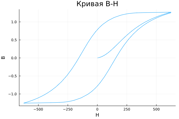
The figure below shows a typical graph of the resulting relationship between and .

In this case, at the initial moment of time, the magnetization is zero, so the graph starts at . With increasing field strength, the graph tends to an increasing hysteresis curve, and with a change in the rate of change — decreasing. The difference between ascending and descending curves is due to the dependence from the trajectory history. Physically, this behavior corresponds to the fact that the magnetic dipoles in the core align with an increase in field strength, but do not fully return to their original position with a decrease in field strength.

nonlinear reluctance 1

The starting point for the Gills–Atterton equation is to divide the magnetization effect into two parts, one of which is a function of the effective field strength ( ), and the other is an irreversible part that depends on history:

Variable It is called hysteresis-free magnetization because it has no hysteresis. It is described by the following function of the current value of the effective field strength :

This function sets the saturation curve with the limit values. and the saturation point, determined by the value — the shape coefficient of the hysteresis-free curve. Approximately, it can be assumed that it describes the average value of two hysteresis curves. The values are set in the interface of the block by and the dots on the hysteresis-free B-H curve, which are used to determine the values and .

Parameter it is the coefficient of reversibility of magnetization and determines which part of the behavior determines And which one is an irreversible member . In the Gills–Atterton model, the irreversible term is determined by the partial derivative of the field strength:

For , .

A comparison of this equation with the standard first-order differential equation shows that as the field strength increases the irreversible member tries to track a reversible member , but with a variable gain . The gain factor leads to hysteresis at points where changes the sign. The main parameter forming the irreversible characteristic is , which is called the volumetric coupling coefficient. Parameter It is called the inter-domain coupling coefficient and is also used to determine the effective field strength used in constructing a hysteresis-free curve.:

Meaning It affects the shape of the hysteresis loop: as the values increase, the intersection with the B axis shifts upward. However, it should be noted that for stability it is necessary to use a member which should be positive when and negative when . Therefore, not all values are acceptable, the typical maximum value is about 1e−3.

The procedure for finding approximate values of the coefficients of the Gills–Atterton equation

Approximate values for the coefficients of the equation can be determined using the following procedure:

Specify the parameter value Anhysteretic B-H gradient when H is zero ( by ) and a period on a hysteresis-free B-H curve. The values are determined from these values during block initialization and .
Set the value for the parameter Coefficient for reversible magnetization, c, so as to achieve the correct initial value of the derivative B-H when starting the simulation from a point . Meaning approximately equal to the ratio of this initial value of the derivative to Anhysteretic B-H gradient when H is zero. Meaning There should be more 0 And less 1.
Set the value for the parameter Bulk coupling coefficient, K, approximately equal to When on an increasing hysteresis curve.
Start with a very small value and gradually increase it to adjust the value. when crossing the line . Typical values range from 1e-4 before 1e-3. Too large values lead to the fact that the derivative of the B-H curve tends to infinity, which contradicts physics and leads to an error in program execution.

To get a good match with a given B-H curve, you may need to perform these steps several times.

Variables

Use the parameter group Initial Targets to set the priority and initial target values for the block parameter variables before modeling. For more information, see Configuring physical blocks using target values.

Ports

Conserving

# N — The northern terminal
Magnetism

Details

The magnetic port corresponding to the northern terminal of the unit.

Program usage name

port_n

# S — southern terminal
Magnetism

Details

The magnetic port corresponding to the southern terminal of the unit.

Program usage name

port_s

Parameters

Main

# Effective length — effective length of the simulated section
m | um | mm | cm | km | in | ft | yd | mi | nmi

Details

The effective length of the core, i.e. the average length of the magnetic circuit.

The value must be positive and not infinite.

Units	`m` \| `um` \| `mm` \| `cm` \| `km` \| `in` \| `ft` \| `yd` \| `mi` \| `nmi`
Default value	`0.032 m`
Program usage name	`effective_gap`
Evaluatable	Yes

# Effective cross-sectional area — effective cross-sectional area
m^2 | um^2 | mm^2 | cm^2 | km^2 | in^2 | ft^2 | yd^2 | mi^2 | ha | ac

Details

The effective cross-sectional area of the core, i.e. the average area of the magnetic flux path.

The value must be positive and not infinite.

Units	`m^2` \| `um^2` \| `mm^2` \| `cm^2` \| `km^2` \| `in^2` \| `ft^2` \| `yd^2` \| `mi^2` \| `ha` \| `ac`
Default value	`1.6e-05 m^2`
Program usage name	`A_effective`
Evaluatable	Yes

# Averaging period for power logging — the excitation period used for averaging

Details

The averaging period for calculating hysteresis losses. These losses are proportional to the area enclosed in the B-H trajectory. If the unit is excited at a known, fixed frequency, then to calculate the hysteresis losses, this value can be set equal to the corresponding excitation period. In this case, the unit registers hysteresis losses once per AC cycle in the variable power_dissipated. If a fixed-step solver is used, then this value must be an integer multiple of the simulation step size.

If the unit is not energized at a known, fixed frequency, set this parameter to 0. In this case, the block will set the value power_dissipated equal to zero, and you will be able to calculate the actual hysteresis loss by postprocessing the registered variable. power_instantaneous.

Dependencies

This parameter is used if for the parameter Parameterized by value selected Nonlinear reluctance with hysteresis (JA model).

Default value	`0.0`
Program usage name	`averaging_period`
Evaluatable	Yes

B-H Curve

# Parameterized by — The B-H curve parameterization method
Linear reluctance | Reluctance with single saturation point | Reluctance (B-H curve) | Nonlinear reluctance with hysteresis (JA model)

Details

The B-H curve parameterization method.

Values	`Linear reluctance` \| `Reluctance with single saturation point` \| `Reluctance (B-H curve)` \| `Nonlinear reluctance with hysteresis (JA model)`
Default value	`Reluctance (B-H curve)`
Program usage name	`parameterization_option`
Evaluatable	No

# Relative magnetic permeability — relative magnetic permeability

Details

Relative magnetic permeability.

The value must be positive and not infinite.

Dependencies

This parameter is used if for the parameter Parameterized by value selected Linear reluctance.

Default value	`5000.0`
Program usage name	`mu_r`
Evaluatable	Yes

# Unsaturated relative magnetic permeability — relative magnetic permeability

Details

Relative magnetic permeability for an unsaturated inductor.

Dependencies

This parameter is used if for the parameter Parameterized by value selected Reluctance with single saturation point.

Default value	`5000.0`
Program usage name	`mu_r_unsat`
Evaluatable	Yes

# Magnetic flux density at saturation — magnetic induction
T | nT | uT | mT | G

Details

Magnetic induction for a saturated inductor.

The value must be positive and not infinite.

Dependencies

This parameter is used if for the parameter Parameterized by value selected Reluctance with single saturation point.

Units	`T` \| `nT` \| `uT` \| `mT` \| `G`
Default value	`1.5 T`
Program usage name	`B_sat`
Evaluatable	Yes

# Magnetic field strength vector — vector of magnetic field strength values
A/m

Details

Magnetic field strength, , is given as a vector with the same number of elements as in the vector of magnetic induction values, . The vector should start from zero and increase monotonously.

Dependencies

This parameter is used if for the parameter Parameterized by value selected Reluctance (B-H curve).

Units	`A/m`
Default value	`[0.0, 200.0, 400.0, 600.0, 800.0, 1000.0] A/m`
Program usage name	`H_vector`
Evaluatable	Yes

# Magnetic flux density vector — vector of magnetic induction values
T | nT | uT | mT | G

Details

Magnetic induction, , is defined as a vector with the same number of elements as the magnetic field strength vector, . The vector should start from zero and increase monotonously.

Dependencies

This parameter is used if for the parameter Parameterized by value selected Reluctance (B-H curve).

Units	`T` \| `nT` \| `uT` \| `mT` \| `G`
Default value	`[0.0, 1.25, 1.35, 1.44, 1.48, 1.49] T`
Program usage name	`B_vector`
Evaluatable	Yes

# Interpolation option — the interpolation method
Linear | Smooth

Details

The interpolation method that the block uses to determine values at intermediate time points not specified in the preceding vectors.:

Linear — Prioritize computing performance by using a linear function.
Smooth — priority of accuracy due to obtaining a continuous curve with continuous first-order derivatives.

Values	`Linear` \| `Smooth`
Default value	`Linear`
Program usage name	`interpolation_type`
Evaluatable	No

# Anhysteretic B-H gradient when H is zero — derivative of the hysteresis-free B-H curve near zero field strength
H/m | mH/m | nH/m | uH/m | H/km | mH/km

Details

The gradient of the hysteresis-free B-H curve is about zero field strength. It is set as the average value of the gradient of the increasing and decreasing hysteresis curves.

Dependencies

This parameter is used if for the parameter Parameterized by value selected Nonlinear reluctance with hysteresis (JA model).

Units	`H/m` \| `mH/m` \| `nH/m` \| `uH/m` \| `H/km` \| `mH/km`
Default value	`0.0063 H/m`
Program usage name	`dB_dH_0`
Evaluatable	Yes

# Flux density point on anhysteretic B-H curve — the value of magnetic induction at a point on the hysteresis-free curve B-H
T | nT | uT | mT | G

Details

Specify the value of the magnetic induction at a point on the hysteresis-free curve. The most accurate option is to select a point at high field strength, when the increasing and decreasing hysteresis curves coincide.

Dependencies

This parameter is used if for the parameter Parameterized by value selected Nonlinear reluctance with hysteresis (JA model).

Units	`T` \| `nT` \| `uT` \| `mT` \| `G`
Default value	`1.49 T`
Program usage name	`B_anhysteretic`
Evaluatable	Yes

# Corresponding field strength — appropriate field strength
A/m

Details

The corresponding field strength for the point specified by the parameter Flux density point on anhysteretic B-H curve.

Dependencies

This parameter is used if for the parameter Parameterized by value selected Nonlinear reluctance with hysteresis (JA model).

Units	`A/m`
Default value	`1000.0 A/m`
Program usage name	`H_anhysteretic`
Evaluatable	Yes

# Coefficient for reversible magnetization, c — the coefficient of reversibility of magnetization

Details

The proportion of magnetization that is reversible. The value must be greater than zero and less than one.

Dependencies

This parameter is used if for the parameter Parameterized by value selected Nonlinear reluctance with hysteresis (JA model).

Default value	`0.1`
Program usage name	`c`
Evaluatable	Yes

# Bulk coupling coefficient, K — volumetric coupling coefficient
A/m

Details

A parameter of the Gills–Atterton model that determines the magnitude of the field strength at which the B-H curve intersects the line of zero magnetic induction.

Dependencies

This parameter is used if for the parameter Parameterized by value selected Nonlinear reluctance with hysteresis (JA model).

Units	`A/m`
Default value	`200.0 A/m`
Program usage name	`K`
Evaluatable	Yes

# Inter-domain coupling factor, α — the coefficient of inter-domain communication

Details

The Gills–Atterton parameter, which affects the intersection points of curves B-H with the line of zero field strength. Typical values range from 1e−4 before 1e−3.

Dependencies

This parameter is used if for the parameter Parameterized by value selected Nonlinear reluctance with hysteresis (JA model).

Default value	`0.0001`
Program usage name	`alpha`
Evaluatable	Yes