cheby1
Calculation of a type I Chebyshev filter.
| Library |
|
Syntax
Function call
-
b, a = cheby1(n, Rp, Wp)— designs a Chebyshev type I digital low-pass filtern-th order with a normalized bandwidth boundary frequencyWpand the size of the irregularities in the bandwidthRpdB. Functioncheby1returns the coefficients of the numerator and denominator of the filter transfer function.
-
A, B, C, D = cheby1(_; nout=4)— designs a type I Chebyshev digital filter and returns matrices that define its representation in the state space.
-
_ = cheby1(_, "s"; nout)— designs a Type I Chebyshev analog filter using any of the input or output arguments in the previous syntaxes. Argumentnoutshows how many output arguments the function will return. If the argument isnoutomitted, the function will calculate only for the two output arguments.
Arguments
Input arguments
# n — filter order
+
scalar
Details
The filter order, specified as an integer scalar, is less than or equal to 500. For band-pass and notch filters n represents half of the filter order.
| Data types |
|
# Rp is the size of the ripples in the bandwidth in dB
+
positive scalar
Details
The size of the ripples in the bandwidth, set as a positive scalar in dB.
If the value is expressed in linear units, you can convert it to dB using the formula Rp .
| Data types |
|
# Wp — bandwidth limit frequency
+
scalar | two-element vector
Details
The bandwidth boundary frequency, specified as a scalar or two-element vector. The bandwidth cutoff frequency is the frequency at which the amplitude-frequency response of the filter is −Rp in dB. Lower frequency response ripple values in the bandwidth, Rp they lead to increased bandwidth.
-
If
Wp— a scalar, thencheby1designs a low-pass or high-pass filter with a cut-off frequencyWp.If
Wp— two-element vector[w1 w2], wherew1 < w2Thencheby1designs a bandpass or notch filter with a lower cut-off frequencyw1and the upper boundary frequencyw2. -
For digital filters, the bandwidth boundary frequencies should be in the range of
0before1, where1corresponds to the Nyquist frequency — half of the sampling frequency or rad/countdown.For analog filters, the bandwidth boundary frequencies must be expressed in rad/s and can take any positive value.
| Data types |
|
# ftype — filter type
+
"low" | "bandpass" | "high" | "stop"
Details
The filter type specified as:
-
"low"— low-pass filter with bandwidth boundary frequencyWp. This value is used by default for scalarWp; -
"high"— high-pass filter with bandwidth boundary frequencyWp; -
"bandpass"— bandpass filter2nof the order ifWp— a two-element vector. This value is used by default whenWpset as a two-element vector; -
"stop"— notch (blocking) filter2nof the order ifWp— a two-element vector.
| Data types |
|
Name-value input arguments
# nout — number of output arguments
+
2 (by default) | 3 | 4
Details
The number of output arguments, set as 2, 3 or 4. If the argument is nout not specified, the function returns two output arguments by default.
Output arguments
# b, a are the coefficients of the transfer function
+
string vectors
Details
Coefficients of the filter transfer function returned as row vectors. With the specified filter order n the function returns b and a with r by counting where r = n + 1 for low and high pass filters and r = 2 * n + 1 for band-pass and notch filters.
The transfer function is expressed in terms of and :
-
for digital filters
-
for analog filters
| Data types |
|
# z, p, k — zeros, poles, and gain
+
column vectors and scalar
Details
Zeros, poles, and filter gain, returned as two vectors-columns and a scalar. With the specified filter order n the function returns z and p with r by counting where r = n for low and high pass filters and r = 2 * n for band-pass and notch filters.
The transfer function is expressed in terms of , and :
-
for digital filters
-
for analog filters
| Data types |
|
# A, B, C, D — representation of the filter in the state space
+
matrices
Details
The representation of the filter in the state space, returned as matrices. If r = n for low- and high-pass filters and r = 2n for bandpass and notch filters, then A This is the matrix r on r, B the matrix r on 1, C the matrix 1 on r, and D — 1 on 1.
The state space matrices relate the state vector , entrance and the exit by means of systems of equations:
-
for digital filters
-
for analog filters
| Data types |
|
Examples
Chebyshev type I low-pass filter
Details
Let’s design a Chebyshev type I low-pass filter 6-th order with ripples in the bandwidth 10 dB and bandwidth cutoff frequency 300 Hz, which corresponds to 0.6π rad/count for data sampled with frequency 1000 Hz. Let’s plot the amplitude-frequency and phase characteristics. We use it to filter a random signal with a frequency 1000 counts.
import EngeeDSP.Functions: cheby1, freqz, randn, filter

fc = 300
fs = 1000

b, a = cheby1(6,10,fc/(fs/2))

freqz(b,a,out=:plot)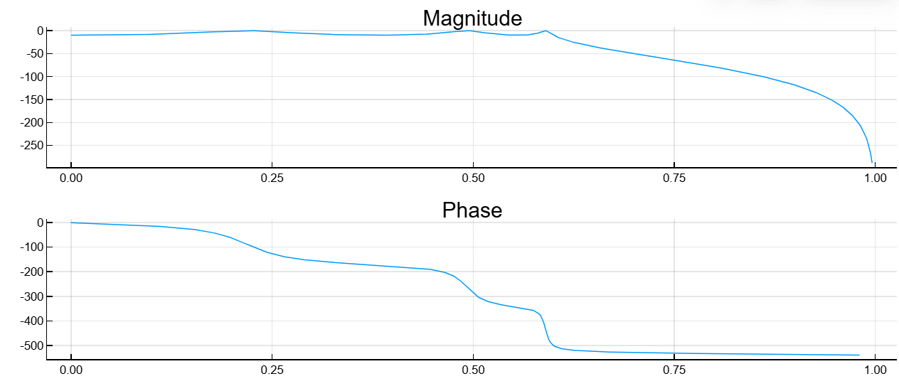
dataIn = randn(1000,1)
dataOut = filter(b,a,dataIn)
Chebyshev Type I barrier filter
Details
Let’s design a type I Chebyshev barrier filter 3-th order with normalized boundary frequencies 0.2π and 0.6π rad/countdown and bandwidth ripples 5 dB. Let’s plot the amplitude-frequency and phase characteristics. We use it to filter a random signal.
import EngeeDSP.Functions: cheby1, freqz, randn, filter

b,a = cheby1(3,5,[0.2 0.6],"stop")

freqz(b,a,out=:plot)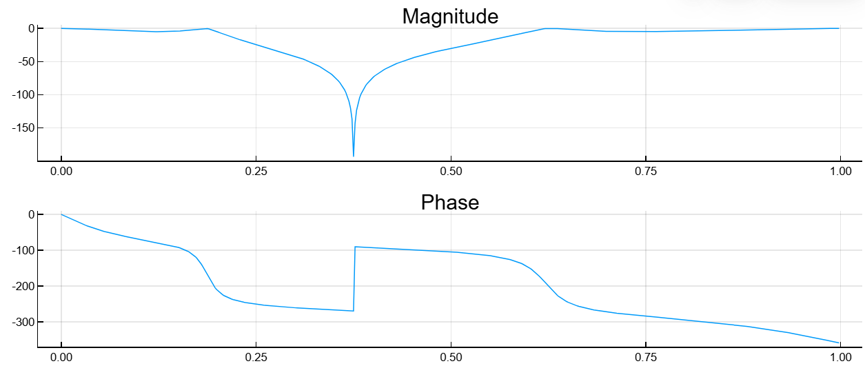
dataIn = randn(1000,1)
dataOut = filter(b,a,dataIn)
Chebyshev type I high-pass filter
Details
Let’s design a Chebyshev type I high-pass filter 9-th order with bandwidth cutoff frequency 300 Hz, which is for data sampled with frequency 1000 Hz, corresponds to 0.6π rad/countdown. Setting the ripple in the bandwidth 0.5 dB. Convert the zeros, poles, and gain into second-order sections. Let’s plot the amplitude-frequency and phase characteristics.
import EngeeDSP.Functions: cheby1, zp2sos

z,p,k = cheby1(9,0.5,300/500,"high"; nout=3)
sos = zp2sos(z,p,k)

freqz(sos,out=:plot)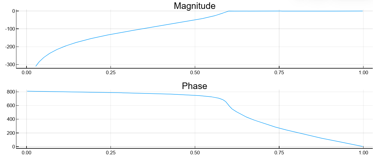
Chebyshev type I bandpass filter
Details
Let’s design a Chebyshev type I bandpass filter 10-th order with lower bandwidth 400 Hz and upper bandwidth 500 Hz. Set the ripple in the bandwidth 3 dB and sampling rate 1500 Hz. We use a representation in the state space. We transform the representation in the state space into the form of sections of the second order. Let’s plot the amplitude-frequency and phase characteristics.
import EngeeDSP.Functions: cheby1, ss2sos
fs = 1500

A,B,C,D = cheby1(10,3,[400 500]/(fs/2); nout=4)
sos = ss2sos(A,B,C,D)[1]

freqz(sos,out=:plot)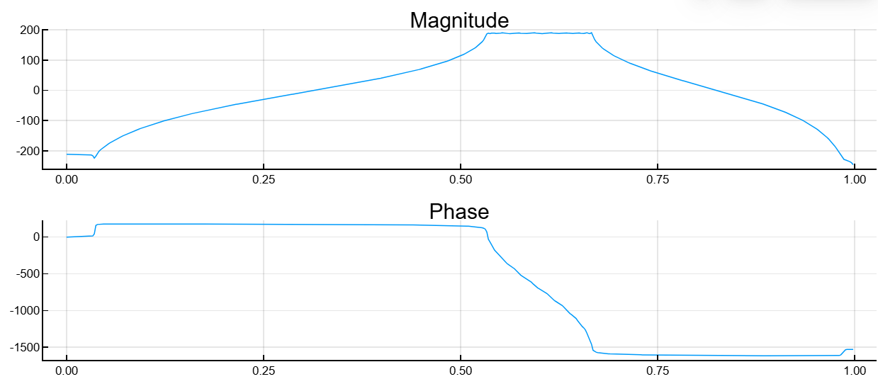
Algorithms
Chebyshev type I filters have a uniform frequency response pulsation in the passband and are monotonous in the delay band. Type I filters have a faster frequency response drop than type II filters, but at the expense of a greater deviation from unity in the bandwidth.
Chebyshev filter type I cheby1 uses a five-step algorithm:
-
Finds the poles, zeros, and gain of the analog low-pass prototype.
-
Converts poles, zeros, and gain into a state space.
-
If necessary, it uses a state space transformation to convert a low-pass filter into a high-pass filter, bandpass filter, or notch filter with the required frequency constraints.
-
To design digital filters, it converts an analog filter to a digital one by means of a bilinear frequency pre-distortion conversion. Fine frequency tuning allows analog and digital filters to have the same frequency response amplitude
Wporw1andw2. -
If necessary, it converts the state space filter back into a transfer function or a zero-pole-gain form.