rangeangle
Calculation of range and slope angle.
| Library |
|
Description
The rangeangle function determines the length and direction of the signal propagation path from a source point or set of source points to a reference point.
The function supports two propagation models - free space model and two-beam model.
-
The free space model represents the line-of-sight trajectory from the source point to the reference point.
-
The two-beam model generates two trajectories. The first trajectory corresponds to the trajectory in free space. The second trajectory represents the trajectory reflected from the boundary plane at . The trajectory directions are defined either with respect to the global coordinate system at the reference point or with respect to the local coordinate system at the control point. Distances and angles at the reference point are independent of the direction in which the signal propagates along the trajectory.
Syntax
Function call
The rangeangle function can be called in the following ways:
-
rng,ang = rangeangle(pos)returns the length of the propagation path (argument rng) and the direction angles (argument and) of the signal path from a source point or set of source points (argument pos) to the origin in the global coordinate system. Direction angles are azimuth and elevation angle relative to the global coordinate axes at the origin. Signals follow a line-of-sight path from the origin to the origin. The line-of-sight path corresponds to a geometric straight line between points. -
rng,ang = rangeangle(pos,refpos)also specifies a reference point or set of reference points (argument refpos). The rng argument now contains the length of the propagation path from the source points to the reference points. The direction angles are the azimuth and elevation with respect to the global coordinate axes at the reference points. Multiple points and multiple reference points can be specified. -
rng,ang = rangeangle(pos,refpos,refaxes)also specifies the local coordinate system axes (argument refaxes) at the reference points. Directional angles are azimuth and elevation with respect to the local coordinate axes with the centre at refpos. -
rng,ang = rangeangle(_,model)also specifies the propagation model. If the model has the valuefreespace, the signal propagates along a line-of-sight path from the source point to the receive point. If the model is set totwo-ray, the signal propagates along two paths from the source point to the receive point. The first path is the line-of-sight path. The second path is the reflective path. In this case, the function returns the distances and angles for the two paths for each source point and the corresponding reference point.
Arguments
Entry
pos -
starting point position
real vector 3 by 1 | real matrix 3 by N
Details
The position of the source point in metres, given as a 3 by 1 real vector or a real matrix 3 by . The matrix represents multiple source points. The columns contain the Cartesian coordinates of the points in the form [x;y;z].
-
If pos is matrix 3 on , we need to specify the input argument refpos as matrix 3 on for the reference points of .
-
If all the anchor points are identical, you can specify the refpos argument as a 3 by 1 vector.
Example: [1000;2000;50].
Data types: Float64
refpos -
reference point position
[0;0;0;0] (by default) | ` real vector 3 by 1` | ` real matrix 3 by N`
Details
The position of a reference point in metres, given as a 3 by 1 real vector or a 3 by real matrix . The matrix represents multiple reference points. The columns contain the Cartesian coordinates of the points in the form [x;y;z].
-
If refpos is matrix 3 at , you must specify the pos argument as matrix 3 at for the source points of .
-
If all the source points are identical, you can specify pos as a 3-by-1 vector.
Example: [100;100;10].
Data types: Float64
refaxes -
axes of the local coordinate system
[1 0 0;0 1 0;0 0 0 1] (by default) | real matrix 3 by 3 | real array 3 by 3 by N
Details
The axes of the local coordinate system, given as a 3-by-3 real matrix or a 3-by-3 array by .
For an array, each page corresponds to a local coordinate axis at each datum.
The columns in the refaxes argument specify the direction of the coordinate axes of the local coordinate system in Cartesian coordinates. must match the number of columns in the pos or refpos argument if these dimensions are greater than one.
Example: rotz(45)
Data types: Float64
model -
distribution model
freespace (by default) | two-rays
Details
A distribution model specified as freespace or two-ray.
-
If
freespaceis specified, the free-space propagation model is invoked. -
If
two-rayis specified, a two-beam propagation model is invoked.
Data types: char, string
Output
rng -
spreading range
real vector 1 over N | real vector 1 over 2N
Details
Propagation range in metres, returned as a vector with real value 1 by or a vector with real value 1 by 2 .
-
If the model argument is set to
freespace, the dimensionality of rng is 1 at . The propagation range is the length of the direct path from the position defined in the pos argument to the corresponding position defined in the refpos argument. -
If the model argument is set to
two-ray, rng contains the ranges for the forward and reflected paths. The alternate columns of rng refer to the line-of-sight path and the reflected path, respectively, for the same source-reference pair.
ang -
azimuth and elevation angles
` real matrix 2 by N` | ` real matrix 2 by 2N`
Details
Azimuth and elevation angles in degrees, returned as a 2 by matrix or a 2 by 2 matrix . Each column represents a direction angle in the form [azimuth;elevation].
-
If the model argument is set to
freespace, the ang argument is a matrix 2 at and represents the path angle from the origin to the reference point. -
If the argument model is set to
two-rays, the argument ang is a 2-by-2 matrix . The alternate columns of ang refer to the line-of-sight path and the reflected path, respectively.
Examples
Calculation of range and slope angle
Details
Calculate the range and tilt angle of a target located at a distance of (1000,2000,50) metres from the origin.
TargetLoc = [1000;2000;50];
tgtrng,tgtang = rangeangle(TargetLoc)
Calculation of range and tilt angle with respect to local coordinates
Details
Calculate the range and angle to a target located at a distance of (1000,2000,50) metres but relative to the origin in a local coordinate system at a distance of (100,100,10) metres. Select a local coordinate reference system that is rotated about the axis by 45° relative to the global coordinate axes.
targetpos = [1000;2000;50];
origin = [100;100;10];
refaxes = [1/sqrt(2) -1/sqrt(2) 0; 1/sqrt(2) 1/sqrt(2) 0; 0 0 1];
tgtrng,tgtang = rangeangle(targetpos,origin,refaxes)
Additional Info
Angles in local and global coordinate systems
Details
The rangeangle function returns the distance to the trajectory and the angles of the trajectory in global or local coordinate system.
Each antenna or acoustic element and antenna array has a radiation pattern, which is expressed in local angular coordinates of azimuth and elevation.
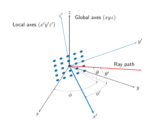
When the element or antenna array moves or rotates, the gain pattern is carried along with it. To determine the signal strength, you must know the angle that the signal path makes with respect to the local angular coordinates of the element or antenna array. By default, the rangeangle function defines the angle that the signal path makes to the global coordinates.
If you add the refaxes argument, you can calculate angles with respect to local coordinates. As an illustration, this figure shows a 5 by 5 uniform rectangular array (URA) rotated with respect to global coordinates ( ) using refaxes. The axis of the local coordinate system ( ) is aligned with the major axis of the array and moves as it moves. The path length is independent of orientation. The global coordinate system defines azimuth angles and elevation angles ( , ), and the local coordinate system defines azimuth angles and elevation angles ( , ).
Local and global coordinate axes
Free space propagation model
Details
The free-space propagation model states that a signal propagating from one point to another in a homogeneous, isotropic medium travels along a straight line called the line of sight, or straight ray.
The straight line is defined by the geometric vector from the source of radiation to the destination. Similar assumptions are made for sonar, but instead of the term "free space" the term isotropic channel is used.
Two-beam propagation model
Details
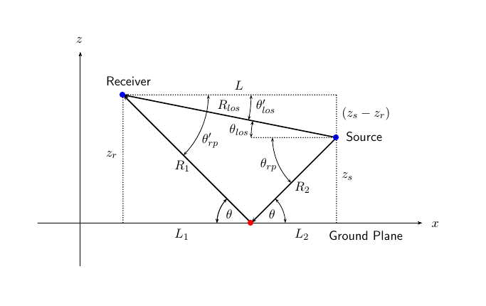
The two-beam propagation channel is the next step in complexity after the free-space channel and is the simplest case of a multibeam propagation medium. The free-space channel models a rectilinear path by line of sight from point 1 to point 2. In a two-beam channel, the medium is defined as a homogeneous, isotropic medium with a reflective planar boundary. The boundary is always set to = 0. There are at most two rays propagating from point 1 to point 2. The first ray propagates along the same line-of-sight trajectory as in the free space channel. The line-of-sight trajectory is often called the direct trajectory. The second ray reflects off the boundary before reaching point 2.
According to the law of reflection, the angle of reflection is equal to the angle of incidence. In short-range simulations, such as cellular telephone systems or car radars, we may assume that the reflecting surface, the ground or ocean surface, is flat.
The figure shows two propagation paths. From the source position, , and the receiver position, , you can calculate the angles of arrival for both paths, and .
The angles of arrival are the elevation and azimuth angles of the incoming radiation with respect to the local coordinate system. In this case, the local coordinate system is the same as the global coordinate system.
You can also calculate the transmission angles, and . In global coordinates, the reflection angle at the boundary coincides with the angles and .
The reflection angle is important to know when you use angle-dependent reflection loss data. You can determine the reflection angle by using the rangeangle function and setting the reference axes to a global coordinate system. The total path length for the line-of-sight path is shown in Figure , which is equal to the geometric distance between the source and receiver. The total path length for the reflected trajectory is . The value is the distance between the source and the receiver.
You can easily derive exact formulas for path lengths and angles in terms of distance to the ground and height of objects in a global coordinate system.