Image synthesis for an optical system
In this example, we will create a test video for an optical sensor by combining a number of synthesized images of a visual target. The motion model will be set in the form of an Engee dynamic model, and we will perform all the processing in a script.
Organizing the video synthesis process
Synthetic images are needed to debug optical system models. In this demo, we synthesize such an image for a motion model defined using graphic blocks in a file. aero_vibration.engee.
We will create a 64-by-64-pixel image and save an 80-frame video (at 10 frames per second).
The image will consist of a target set against a moving background, and the observation point will be subject to random vibration. The pattern of movement of the observation point will be set by the model. aero_vibration attached to the example. In addition, the image will be blurred using a Gaussian filter (as a dot scattering function).
Pkg.add( ["Interpolations"] )
delt = 0.1;      # The sampling period of the model
num_frames= 140;  # The number of frames to synthesize
framesize = 64;  # The size of the image side in pixels

# Let's create a 3D matrix to store a stack of 2D images along a time vector
out = zeros( framesize, framesize, num_frames);
Creating a target and its motion model
First of all, we will define the appearance of the target and the model of its movement. We chose a noticeable plus sign as a target, and the resulting matrix stores the intensity values of its pixels. According to the specified motion model, the target will move from the center of the image to its lower right corner.
target = [zeros(3,11)
          zeros(1,5) 6 zeros(1,5)
          zeros(1,5) 6 zeros(1,5)
          zeros(1,3) 6 6 6 6 6 zeros(1,3) # As a target, we'll draw a 5-by-5 plus sign.,
          zeros(1,5) 6 zeros(1,5)         # intensity 6 is selected for the sake of the signal-to-noise ratio of ~4
          zeros(1,5) 6 zeros(1,5)         # We make the target image a little bigger (11x11 pixels)
          zeros(3,11)];                   # to work with this image without interpolation errors

target_velx = 1;                  # the speed of the target along the X-axis (pixels/sec)
target_vely = 1;                  # the speed of the target along the Y-axis (pixels/sec)
target_x_initially = framesize÷2; # initially, the target is located in the center of the image on both axes
target_y_initially = framesize÷2; # x and y

gr()
heatmap( target.*32,
         c=:grays, framestyle=:none, aspect_ratio=:equal, leg=:false,
         title="Target image" )
Combining the target image and background
Let's create a background of two sinusoids and set a model of its movement. Then we will overlay the image of the target on top of it.
using FFTW

backsize = framesize+36;  # The background image is significantly larger than the target image
                          # Because we don't want to lose sight of the target as we move.
xygrid = (1:backsize) ./ backsize;
B = (2sin.(2pi .* xygrid).^2) * (cos.(2pi .* xygrid).^2)';

psd = fft( B );
psd = real( psd .* conj(psd) );

background = B .+ 0.5*randn(backsize, backsize);    # Add Gaussian noise
					                                # with a variation of 0.25 (COE 0.5)

xoff = 10;     # The initial displacement of the sensor origin point
yoff = 10;     # relative to the point (0,0) of the background image

driftx = 2;    # Background image displacement rate (pixels/sec)
drifty = 2;

minout = minimum( background );
maxout = maximum( background );

heatmap( (background.-minout) .* 64 ./ (maxout.-minout),
         c=:grays, framestyle=:none, aspect_ratio=:equal, leg=:false, clim=(0,255),
		 title="Background image + noise" )
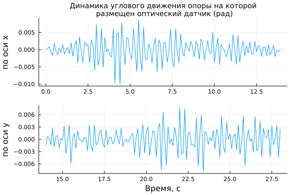
We simulate the angular vibration of the camera
The vibration of the sensor is expressed in the displacement of the camera image. The time series that defines the camera vibration description is calculated in the model aero_vibration.
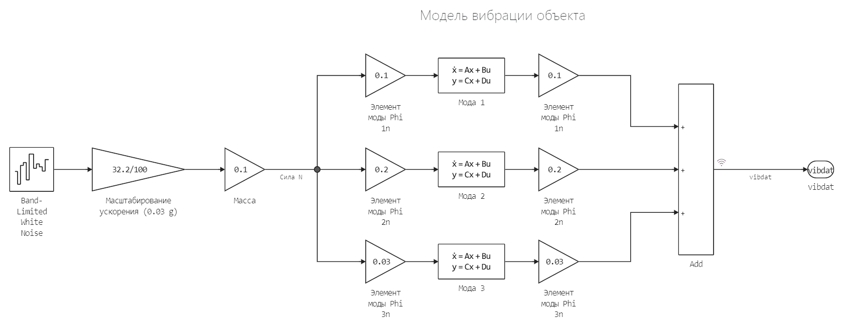
We will run the model using software control commands (variable delt set at the beginning of this example).
omega = 2*pi*5;       # The vibration of the structure consists of vibrations of 5, 10 and 15 Hz
zeta  = 0.01;         # Damping coefficient for all components (mod)

# Open and execute the model
modelName = "aero_vibration";
model = modelName in [m.name for m in engee.get_all_models()] ? engee.open( modelName ) : engee.load( "$(@__DIR__)/$(modelName).engee");
engee.set_param!( modelName, "FixedStep"=>delt );
engee.set_param!( modelName, "StopTime"=>num_frames*delt*2 );

data = engee.run( modelName, verbose=false );

# The result of running the model is divided into two vectors
vibtime = data["vibdat"].time
vibdata = data["vibdat"].value
vibLen = length( vibdata )

vibx = vibdata[ 1:vibLen÷2 ]
viby = vibdata[ (vibLen÷2+1):end ]

levarmx = 10;   # The length of the lever that converts rotational vibration into longitudinal motion
levarmy = 10;   # on the X and Y axes

plot(
    plot( vibtime[1:vibLen÷2], vibx, title="Dynamics of angular motion of the support on which the optical sensor (rad) is placed",
           ylabel="on the x-axis", grid=true, titlefont=font(10), leg=:false ),
    plot( vibtime[(vibLen÷2+1):end], viby, xlabel="Time, from", ylabel="on the y axis", grid=true, leg=:false ),
    layout=(2,1)
)
We simulate movement in the frame by combining background, target, and vibration.
Now we will synthesize all the frames of the future video and put them into the matrix. out. All frames will be different because the image is formed from a moving target and background, and the camera vibrates. Below we will show the first frame of this video.
using Interpolations

for t = 1:num_frames

    # Shifting the background at driftx and drifty speeds and adding vibration
    xshift = driftx*delt*t + levarmx * vibx[t];
    yshift = drifty*delt*t + levarmy * viby[t];

    # Background image interpolation (subpixel image movement)
    x2,y2 = ( xshift:1:xshift+backsize, yshift:1:yshift+backsize )
    itp = LinearInterpolation((1:backsize, 1:backsize), background, extrapolation_bc=Line())
    outtemp = [ itp(x,y) for y in y2, x in x2 ]

    # Cropping an image to the framesize size (from the backsize size)
    out[:,:,t] = outtemp[xoff:xoff+framesize-1, yoff:yoff+framesize-1];

    # Add target movement
    tpixinx = floor( target_velx * delt * t );  # Saving the displacement amplitude before interpolation
    tpixiny = floor( target_vely * delt * t );  # in whole pixels

    # Interpolation of brightness values
    txi = target_velx*delt*t - tpixinx;
    tyi = target_vely*delt*t - tpixiny;
    txi,tyi = ( txi+1:txi+11, tyi+1:tyi+11)     # The target needs to be interpolated only relative to its center

    itp = LinearInterpolation( (1:11, 1:11), target, extrapolation_bc=Line() )
    temp = [ itp(x,y) for y in tyi, x in txi ]

    # Place the target image at a point defined by the initial camera offset and the previously stored offset amplitude
    tx = convert(Int64, tpixinx + target_x_initially - 1);
    ty = convert(Int64, tpixiny + target_y_initially - 1);

    out[tx:tx+6, ty:ty+6, t] = temp[9:-1:3, 9:-1:3] + out[tx:tx+6,ty:ty+6,t];

end

minout = minimum( out );
maxout = maximum( out );

heatmap( (out[:,:,1].-minout) .* 64 ./ (maxout.-minout),
         c=:grays, framestyle=:none, aspect_ratio=:equal, leg=:false, clim=(0,255),
		 title="Combined image" )
Optical system model (Gaussian "diaphragm model")
The optical system model here boils down to frequency domain image blurring (FFT). There are simpler ways to solve this problem (apply a blur). But the method proposed here allows you to implement a much more complex "aperture model" – you only need to replace the first 5 lines of the next cell with your function.
x = 1:framesize;
y = 1:framesize;
sigma = 120;
apfunction = @. exp(-(x-framesize/2).^2/(2*sigma))' * exp(-(y-framesize/2).^2/(2*sigma));
apfunction = fftshift(apfunction);

for j = 1:num_frames
    out[:,:,j] = real.( ifft( apfunction.*fft( out[:,:,j] )));
end

minout = minimum(out);
maxout = maximum(out);

heatmap( (out[:,:,1].-minout) .* 64 ./ (maxout.-minout),
         c=:grays, framestyle=:none, aspect_ratio=:equal, leg=:false, clim=(0,255),
		 title="Blurred image" )
Creating and playing a video clip
Finally, we scale the image so that the pixel intensity value is between 0 and 64 and output a video clip.
minout = minimum(out);
maxout = maximum(out);

a = Plots.Animation()

for j = 1:num_frames
    plt = heatmap( (out[:,:,j] .- minout)*64/(maxout-minout),
        c=:grays, framestyle=:none, aspect_ratio=:equal, leg=:false, clim=(0,255),
        size=(400,400), yflip=true )
    frame( a, plt )
end

gif( a, "1.gif", fps=15 )
Let's draw another graph to compare the brightness levels of the object and the background, speeding up the visualization a little.
a = Plots.Animation()

for j = 1:num_frames
    plt = wireframe( (out[:,:,j] .- minout)*64/(maxout-minout),
        c=:grays, aspect_ratio=:equal, leg=:false,
        size=(500,500), yflip=true, zlimits=(0,64), grid=true )
    frame( a, plt )
end

gif( a, "2.gif", fps=15 )
Conclusion
We have successfully synthesized a small video on which we can test some task for the optical system – tracking or object recognition. The model of the object's movement was set by us using several graphic blocks, and image synthesis was performed in an interactive script.