A model of a missile with a homing system
We will show how to add a model of a homing system to the rocket model, which will be triggered when a target is detected and bring the control object to the desired point in space.
The model of object dynamics
The control object is a rocket of a normal aerodynamic design with wings in the middle and rudders in the tail section.
The main part of the object model is a nonlinear representation of rigid body dynamics (block 3DOF (Body Axes)The aerodynamic forces and torques acting on the rocket body are calculated based on coefficients that are represented by a nonlinear dependence on both the Mach velocity and the angle of attack. These functions are stored in the model in tabular form, in blocks. 2-D Lookup Table.
The model uses the following blocks from the "Aerospace Systems" palette, which are standard for all aerospace systems (for example, the standard atmosphere model).
.png)
Description of the airframe model
The dynamic glider model consists of four main subsystems and an autopilot, which controls the normal acceleration of the rocket by moving the rudder. Subsystem Atmosphere, Angle of attack and Airspeed calculates the effect of atmospheric conditions depending on the flight altitude. Subsystems The steering wheel drive and Sensors link the autopilot model to the airframe model. The block Aerodynamic Forces and Motion Model calculates the forces and torques acting on the rocket body, and then calculates the motion model.
.png)
Atmosphere and airspeed
This model uses a standard block ISA Atmosphere Model - The ISA Standard Atmosphere Model (ISA). In additional blocks, the speed (in Max) is calculated using the current speed of sound, as well as the velocity pressure. Q.
.png)
Aerodynamic forces and coefficients
The Aerodynamic forces subsystem calculates the forces and moments applied to the rocket in the axes of the body. Then the equations of motion are integrated, which determine the linear and angular motion of the control object.
.png)
The aerodynamic coefficients are stored in tabular form, and the instantaneous values during the simulation are determined by interpolation.
.png)
Autopilot model
The rocket's autopilot controls the elevator based on a preset normal acceleration. The accelerometer is placed closer to the nose of the rocket, ahead of the center of gravity. Its signal, with additional damping, is used to generate a control signal.
Autopilot coefficients were selected based on several linearized airframe models obtained for different flight conditions in the expected range. The model also includes a saturation control channel (anti-windup) to prevent the regulator from saturating when the autopilot signal goes beyond the acceptable values.
We are testing the autopilot created in this way in the nonlinear model presented in this project.
The outline of the guidance
Two subsystems are responsible for target detection and tracking:
- The tracking system returns an estimate of the current relative motion parameters between the missile and the target
- The guidance system calculates the desired normal acceleration in pursuit mode and the desired viewing angle in search mode
.png)
Guidance System Calculator
This subsystem provides control signals for different systems.:
- A self-destruct signal when more than the specified time has passed since the target was captured.,
- Set viewing angle in target search mode,
- a fixed command for normal acceleration in the "blind flight" mode (final mode),
- actually, the operating mode of the system,
- a signal to remove the fuse from the system.
.png)
Latin names are usually needed as a compromise for the correct operation of the code generator.
The computer controls the operation of all on-board systems through a variable Mode (external variable Режим). This variable is responsible for switching control modes. During target search, the calculator directly controls the angle of the line of sight by sending a signal Sigma_d on the antenna suspension. When the target is within the capture radius of the seeker beam (signal Acquire or Захват), the system performs a preset pause, and then switches to closed-loop tracking mode. In case of possible ** loss of capture **, the system first switches to search mode, and after a designated time, self-destruction occurs.
The first state machine issues control commands for movement and tracking, and also transmits a signal to the second machine. id_timeout if the allowed pursuit time is exceeded after the loss of the target:
.png)
The second machine outputs a safety release signal when the target is approaching (if the system is in standby mode RadarGuided or if the waiting time is exceeded.
.png)
Proportional control in tracking mode
After the seeker captures the target and up to a collision (or self-recurrence), a proportional control law is used to control the missile. This control law calculates the desired normal acceleration based on the following data:
- measurement of the approach velocity of the missile and the target, which can be obtained using a Doppler tracking device if the homing head is equipped with radar equipment,
- estimation of the rate of change of the line of sight angle (scanning speed).
.png)
The tracking subsystem
This subsystem detects and tracks the target, controls the orientation of the antenna and its retention on the target according to the control law. Time constant of the tracking contour tors It is equal to 0.05 seconds, its setting allows you to set a balance between the desired reaction speed and noise resistance. The stabilization loop is responsible for correcting the speed of the antenna beam displacement to account for the angular velocity of the housing. Its coefficient is selected based on the gyroscope bandwidth.
At the output, the system, in addition to state variables, outputs an estimate of the angular velocity of the target - a smoothed sum of the speed of movement of the antenna beam and the rate of change of the antenna-target angle received from the radar. The bandwidth of the filter is equal to half the bandwidth of the autopilot.
.png)
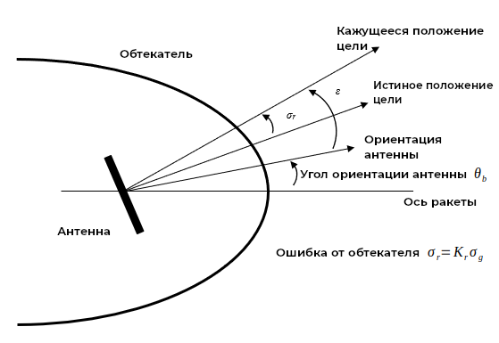
Fairing error
For radar-guided missiles, the fairing is a common source of error, affecting the reception delay and the radiation pattern. As a rule, the magnitude of this error is calculated using a nonlinear function that takes the antenna orientation angle as an input. Our model approximates this effect by a linear relationship between the antenna orientation angle (Gimbal) and the amount of distortion using the "Fairing Error" coefficient.
In this subsystem, models of other important errors can be implemented, for example, the effect of overloads on the operation of gyroscopes. These models will allow you to check the reliability of the regulators of the tracking and stabilization circuit.
.png)
Launch and demonstration of the system
Now let's run the model for execution. The following initial parameters are set in its Callbacks:
- the target is moving at a constant speed of 328 m/s on a collision course
- The target is 500 m below the antenna launch point
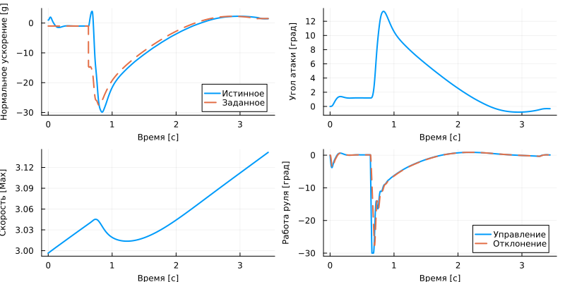
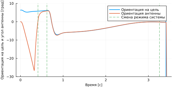
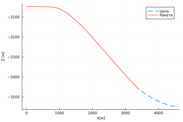
The result shows that the capture occurs 0.42 seconds after launch, then at 0.63 the system switches to tracking mode, and the collision occurred at 3.27 seconds.
include("$(@__DIR__)/init_params.jl")

engee.open("$(@__DIR__)/aero_guidance.engee")
res = engee.run("aero_guidance");
Let's separate the necessary signals:
Mach_speed = collect(res["Atmosphere, Angle of Attack, and Airspeed.Speed (Max)"]);
sigma_antenna = collect(res["Tracking and evaluating the scanning speed.Antenna orientation"]);
sigma_target = collect(res["Goal orientation.1"]);
sigma_rad = collect(res["Sigma_rad"]);
alpha = collect(res["Incidence & Airspeed.α"]);
mode = collect(res["Guidance system computer (100 Hz).Mode"]);
misile_traj = collect(res["Glider and Autopilot.Xe,Ze"]);
target_traj = collect(res["The position of the target.Goal"]);
Az = collect(res["Aerodynamic forces and Motion model.Ax,Az"]);
Az_d = collect(res["Az_d.1"]);
fin_demand = collect(res["Autopilot.Preset steering position"]);
fin_position = collect(res["Steering wheel drive.B"]);
model_stop = collect(res["Undermining.Stop"]);
Let's plot the state variables and visualize the trajectories.:
gr()
plot(
    plot( Az.time, [last.(Az.value) Az_d.value]./9.81, ls=[:solid :dash], ylabel="Normal acceleration [g]", label=["True" "Given"], xlabel="Time [c]" ),
    plot( alpha.time, rad2deg.(alpha.value), ylabel="Angle of attack [deg]", xlabel="Time [c]", leg=false ),
    plot( Mach_speed.time, Mach_speed.value, ylabel="Speed [Max]", xlabel="Time [c]", leg=false ),
    plot( fin_demand.time, rad2deg.([fin_demand.value fin_position.value]), ls=[:solid :dash], ylabel="Steering wheel operation [hail]", label=["Management" "Deviation"], xlabel="Time [c]" ),
    guidefont=font(8), lw=2, size=(800,400)
)
mode_change_idx = findall( diff(mode.value).>0 )

plot( sigma_target.time, rad2deg.(sigma_target.value), label="Goal orientation", ylimits=(-30,10), lw=2 )
plot!( sigma_antenna.time, rad2deg.(sigma_antenna.value), label="Antenna orientation", ls=[:solid :dash], lw=2 )
vline!( [mode.time[mode_change_idx]], ls=:dash, label="Changing the system mode" )
plot!( guidefont=font(8), lw=2, size=(600,300), xlabel="Time [s]", ylabel="Target orientation and antenna angle [deg]" )
plot( first.(target_traj.value), last.(target_traj.value), label="Goal", lw=2, ls=:dash )
plot!( first.(misile_traj.value), last.(misile_traj.value), label="Rocket", lw=2 )
plot!( guidefont=font(8), size=(600,400), xlabel="X[m]", ylabel="Z [m]" )
Now it is easy to run the model for any set of input conditions and study its operation.
Conclusion
We have implemented a relatively complex model of the missile guidance system and traced its trajectory.
[2] Lebedev A.A., Chernobrovin L. S. Flight dynamics of unmanned aerial vehicles, Moscow, 1973.