Creating a seq2seq model for a regression task
In this example, we will train a deep neural network to predict the remaining life of a gas turbine engine.
Downloading and unpacking data
The CMAPSSData open dataset stores simulated engine operation data.: 100 training examples and 100 validation examples. The training data contains a time series consisting of a sequence of measured parameters recorded from startup to failure. The validation data is terminated before the failure event occurs.
Each row contains 26 variables.:
- 1: Engine number
- 2: Operating time (in cycles)
- 3-5: Engine settings
- 6-26: Sensor measurements 1-21
Let's prepare the working environment and upload the dataset.
Pkg.add(["Statistics", "DelimitedFiles", "JLD2", "Flux"])
using DelimitedFiles
dataTrain = Float32.( readdlm( "CMAPSSData/train_FD001.txt" ));
Prepare the training data
As a result of this processing, we will get arrays XTrain and YTrain, containing time series consisting of features (predictors, predictors) and target variables (targets, targets).
function dataPreparation( dataTable )
    numObservations = maximum( dataTrain[:,1] )

    predictors = []
    responses = []

    for i ∈ 1:numObservations
        idx = dataTable[:,1] .== i
        push!( predictors, dataTable[idx, 3:end] )
        timeSteps = dataTable[idx,2]
        push!( responses, reverse(timeSteps) )
    end

    return predictors, responses
end
XTrain, YTrain = dataPreparation( dataTrain );
Remove constant signs
Immutable features don't add anything to our learning process, so we'll get rid of them to speed up calculations. Namely, we will delete the columns from the dataset, where the minimum and maximum are the same values.
m = [ minimum( table, dims=1 ) for table in XTrain ];
M = [ maximum( table, dims=1 ) for table in XTrain ];
idxConstant = [ m[i] .== M[i] for i in 1:length(m) ];
constant_features = vec( maximum( vcat(idxConstant...), dims=1 ) );
XTrain = [ xtrain[:, .!constant_features] for xtrain in XTrain  ];
numFeatures = size( XTrain[1], 2 )
There are 16 signs left for each observation (it is worth remembering that all observations have different lengths, each engine has run a different number of cycles before failure).
Normalization of feature values
Another technique that usually speeds up learning is to prepare the signs by giving each series a mathematical expectation of 0 and a variance of 1. We will collect the signals from all the engines in one column.
using Statistics

mu = vec(mean( vcat([xtrain for xtrain in XTrain]...), dims=1 ));
sig = vec(std( vcat([xtrain for xtrain in XTrain]...), dims=1 ));

XTrain = [ mapslices(row -> (row .- mu) ./ sig, xtrain; dims=2) for xtrain in XTrain ];
gr()
plot(
    heatmap( XTrain[1], cbar=false, yflip=true, title="Observations (predictors)", ylabel="Time (cycles)" ),
    heatmap( reshape(YTrain[1],:,1), yflip=true, title="Target variable: remaining resource (target)" ),
    size=(800,400)
)
plot!( titlefont = font(9) )
Limitation for the output variable
We will predict one number – the number of work cycles remaining before failure. It is more important for us that the predictions are more accurate towards the end of the life cycle.
Therefore, we will limit the predicted variable from above to a resource of 150 operating cycles per failure.
thr = 150
YTrain = [ min.(ytrain, 150) for ytrain in YTrain ];
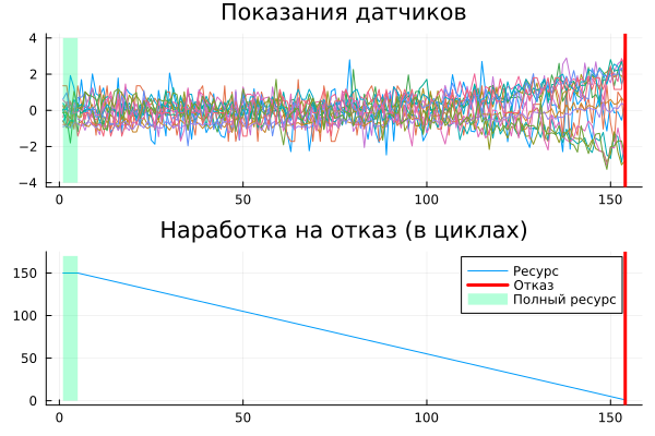
This is what the sensor readings for some engine in the dataset look like.
obs_id = 77

dl = size( XTrain[obs_id], 1 );
cl = maximum( findall( YTrain[obs_id] .== thr ))

a = plot( XTrain[obs_id], leg=:false, title="Sensor readings", label=:none )
vline!(a, [dl], lw=3, lc=:red, label=:none )
plot!(a,  [1, cl], [-4,-4], fillrange=[4,4], fillcolor=:springgreen, fillalpha=0.3, linealpha=0.0, label=:none )

b = plot( YTrain[obs_id], title="Operating time to failure (in cycles)", label="Resource" )
vline!(b, [dl], lw=3, lc=:red, label="Refusal" )
plot!(b,  [1, cl], [0,0], fillrange=[thr+20,thr+20], fillcolor=:springgreen, fillalpha=0.3, linealpha=0.0, label="Full resource" )

plot(a, b, layout=(2,1) )
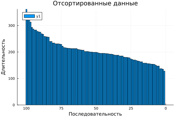
Let's sort the data
This is an optional step. Sometime it will help us split the data into more optimal batches, but first we just need to find out what the length of the largest sequence in the sample is.
# Arrange data by size
sequenceLength = [ size(xtrain,1) for xtrain in XTrain ];
idx = sortperm( sequenceLength, rev=true );
XTrain = XTrain[idx];
YTrain = YTrain[idx];
bar( sort(sequenceLength), xlabel="Sequence", ylabel="Duration", title="Sorted data", xflip=true)
Neural network architecture
We will train two recurrent neural networks and compare the results.:
- RNN neural network (a regular recurrent layer, followed by several fully connected ones)
- LSTM neural network (instead of the basic recurrent layer, a slightly more complex, LSTM layer, the remaining layers are the same)
Before updating the library
Fluxuntil the latest version, the following code will produce a harmless error messageError during loading of extension DiffEqBaseZygoteExt...which does not interfere with work. Just right-click on it and selectУдалить выбранное.
Pkg.add( "Flux" ); # Installing the library in case it is missing
using Flux

numResponses = size( YTrain[1], 2 )
numHiddenUnits = 100
numHiddenUnits2 = 40

rnn = Chain(
    RNN(numFeatures => numHiddenUnits),
    Dense(numHiddenUnits => numHiddenUnits2),
    Dropout(0.5),
    Dense(numHiddenUnits2 => numResponses)
) |> f32;

lstm = Chain(
    LSTM(numFeatures => numHiddenUnits),
    Dense(numHiddenUnits => 50),
    Dropout(0.5),
    Dense(50 => numResponses)
) |> f32;
Let's remember these two neural networks in the state they were in before the start of training, so that we can compare them with trained networks later.
rnn_empty = deepcopy(rnn);
lstm_empty = deepcopy(lstm);
Learning cycles
First, we will train the RNN neural network.
epochs = 100;
The training time of this network before the 100th epoch will be 5-7 minutes.
using JLD2
if !isfile( "rnn.jld2" )
    model = rnn
    data = zip(XTrain, YTrain)
    opt_state = Flux.setup( OptimiserChain(ClipGrad(1), Adam(1e-2)), model )
    loss( ỹ, y ) = sqrt(Flux.mse( ỹ, y ))

    for epoch ∈ 1:epochs
        print( epoch, " ")
        Flux.train!( model, data, opt_state) do m, x, y
            loss(m(x')', y) # Loss function - error on each element of the dataset
        end
    end

    # Save the resulting neural network to a file
    jldsave("rnn.jld2"; rnn);
end
For comparison, we will train an LSTM neural network (* be careful, the training time up to the 100th epoch may exceed 15 minutes*). Let's also add that the number of neurons in the hidden layers, of course, affects the learning time, but not as much as the number of epochs.
if !isfile( "lstm.jld2" )
    model = lstm
    data = zip(XTrain, YTrain)
    opt_state = Flux.setup( OptimiserChain(ClipGrad(1), Adam(1e-2)), model )
    loss( ỹ, y ) = sqrt(Flux.mse( ỹ, y ))

    for epoch ∈ 1:epochs
        print( epoch, " ")
        Flux.train!( model, data, opt_state) do m, x, y
            loss(m(x')', y) # Loss function - error on each element of the dataset
        end
    end

    jldsave("lstm.jld2"; lstm); # Saving the neural network
end
It is believed that LSTM neural networks can "internalize" longer-term dependencies than RNNs.
In conventional recurrent neural networks, the influence of recent measurements on the result is always higher than * the influence of earlier measurements*.
That is, RNNs tend to "forget the distant past". But, on the other hand, the LSTM neural network learned 2-3 times slower than the RNN due to the larger number of equations in each neuron.
Checking the results
Neural networks are pretty good at predicting training data:
using JLD2
@load "rnn.jld2" rnn
@load "lstm.jld2" lstm

test_id = 6

xi = XTrain[test_id]
yi = YTrain[test_id]

# Forecasts before training
y_pred_rnn_empty = rnn_empty(xi');
y_pred_lstm_empty = lstm_empty(xi');

# # Forecasts after training
y_pred_rnn = rnn(xi')
y_pred_lstm = lstm(xi')

plot(
    plot( [y_pred_rnn_empty' y_pred_lstm_empty'], label=["rnn" "lstm"], title="Forecasts before training", lw=2 ),
    plot( [y_pred_rnn' y_pred_lstm' yi], label=["rnn" "lstm" "truth"], title="Forecasts of the trained neural network", lw=2 ),
    size=(800,300), titlefont=font(11)
)
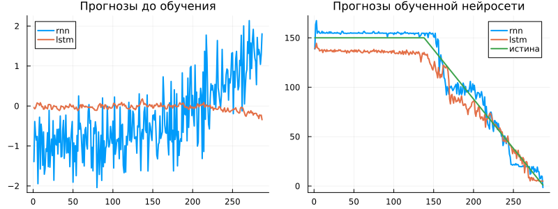
As we have seen, before training, the neural network always gave forecasts close to zero. After training, she learned how to associate a vector of 16 dimensions with a scalar forecast of the remaining resource. It can be assumed that the model takes into account the background of the process, since there is always a downward trend in the forecast, despite the rather chaotic behavior of the signal.
Let's study the forecasts for the training sample.
function get_plot(id)

    xi = XTrain[id]
    yi = YTrain[id]

    Flux.reset!( rnn )  # Reset the state of the neural network so that the accumulated information
    Flux.reset!( lstm ) # the difference from past runs did not affect future forecasts

    y_pred_rnn = rnn(xi');
    y_pred_lstm = lstm(xi');

    return plot( [y_pred_rnn' y_pred_lstm' yi], legend=false, lw=2, title="Forecasts for the sample #$id" )
end

plot( get_plot.(1:16)..., titlefont=font(7), size=(800,600) )
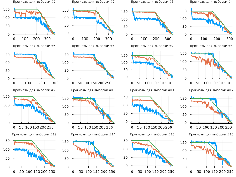
You can see that based on the LSTM test data, the neural network has learned to determine the beginning of the resource well and track the dynamics to the end. But the non-linearity of the learned characteristic is more often manifested in the learning outcomes of the RNN neural network (the hump in the middle of the function).
Let's prepare the test data:
dataTest = Float32.( readdlm( "CMAPSSData/test_FD001.txt" ));
XTest, YTest = dataPreparation( dataTest );
XTest = [ xtest[:, .!constant_features] for xtest in XTest  ];
mu = vec(mean( vcat([xtest for xtest in XTest]...), dims=1 ));
sig = vec(std( vcat([xtest for xtest in XTest]...), dims=1 ));
XTest = [ mapslices(row -> (row .- mu) ./ sig, xtest; dims=2) for xtest in XTest ];

# Addendum: we know the remaining life of the engines in the test sample
YTest = Float32.( readdlm( "CMAPSSData/RUL_FD001.txt" ));
YTest = [ collect((size(XTest[i],1)+(YTest[i])-1):-1:YTest[i]) for i in 1:length(XTest) ];
YTest = [ min.(YTest[i], 150) for i in 1:size(YTest,1) ];
Let's see how the models predict the time to failure for one series of measurements from the total sample (on a test sample).
function get_plot( id )

    xi = XTest[id]
    yi = YTest[id]

    Flux.reset!( rnn )  # Reset the state of the neural network so that the accumulated information
    Flux.reset!( lstm ) # the difference from past runs did not affect future forecasts

    y_pred_rnn = rnn(xi')
    y_pred_lstm = lstm(xi');

    return plot( [y_pred_rnn' y_pred_lstm' yi], legend=false, lw=2, title="Forecasts for the sample #$id", c=[4 6 3] )
end

plot( get_plot.(1:16)..., titlefont=font(7), size=(800,600), legendfont=font(8) )
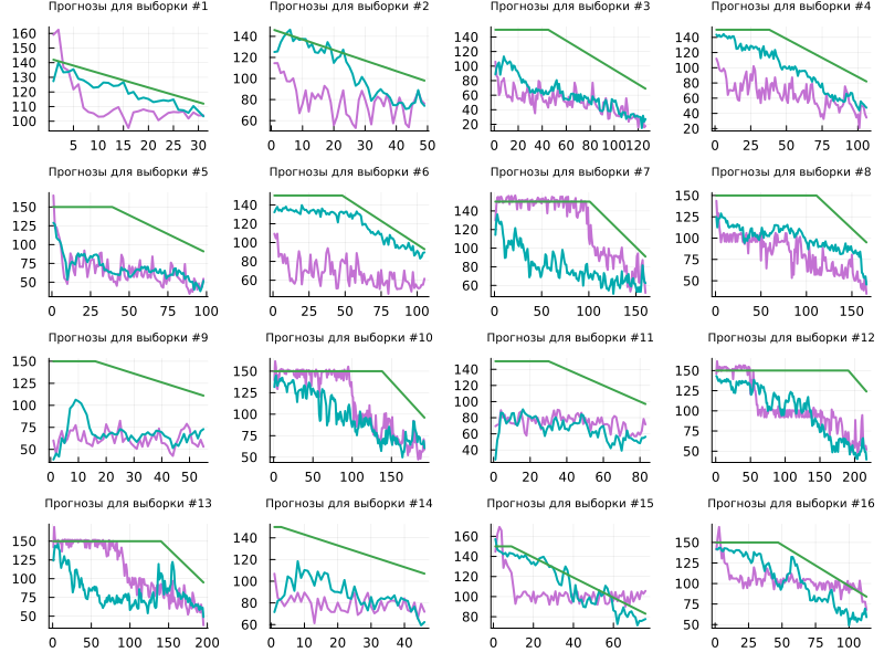
Neural networks perform slightly worse on test data, but it is this information that allows us to choose a further direction for finalizing the architecture and the learning process. As expected, the prediction quality of both neural networks decreases when switching to test data (2.1 times for LSTM and 2.7 times for RNN).
Finally, let's examine the histogram of resource prediction errors at the end of each of the studied lifecycle segments.:
dataset_final_rul = [ ytest[end] for ytest in YTest ]
rnn_final_prediction = [(Flux.reset!( rnn ); rnn(xi')[end]) for xi in XTest]
lstm_final_prediction = [(Flux.reset!( lstm ); lstm(xi')[end]) for xi in XTest]

plot(
    histogram( dataset_final_rul .- rnn_final_prediction, leg=:none, title="RNN prediction error" ),
    histogram( dataset_final_rul .- lstm_final_prediction, leg=:none, title="LSTM forecast error" ),
    size=(900,300), titlefont=font(9)
)
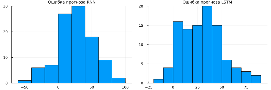
It can be argued that the average error of the LSTM network is closer to 0 than that of the RNN.
We have saved neural networks to files for future reference.
To load them into memory, you will need to download the library first
Flux.
Conclusion
We have trained the neural network to predict the time to failure and now we can assemble a sensor for indirect measurements in order to work it out in the Engee model environment, as well as generate code for the embedded platform and conduct tests in real conditions.
We also note that for educational purposes, in order to speed up the learning process, we implemented a very small neural network and trained it for a fairly small number of cycles. The training of both models took about 10 minutes * in 4 threads on two processors (without GPU)*.