Image processing of the starry sky and obtaining the coordinates of the stars
During this demonstration, we will show the development of an algorithm for detecting the centroids of stars in an image and converting them to a spherical coordinate system.
Engee's modular structure and interactive script editor will allow us to quickly develop a prototype algorithm and evaluate its quality.
Input information for the algorithm
Using photos of the starry sky, we can calculate the orientation of the camera in celestial coordinate systems (for example, экваториальной). At the same time, we will have to create an image processing procedure that is insensitive to various errors inherent in shooting on a mobile platform in low-light conditions. These include thermal sensor noise, blurred images, oversaturated pixels, illumination from external sources, etc.
A useful source of images of the starry sky taken in any conditions is the project's website. https://nova.astrometry.net /
A typical frame from a star sensor looks like this:
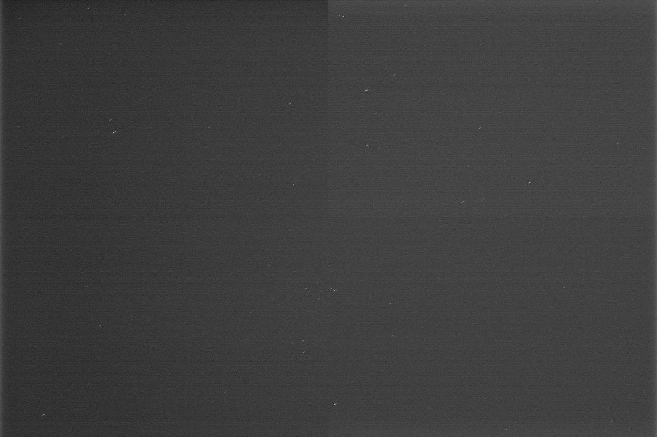
We see a bit of noise, different brightness zones (sensor or primary processing errors), and motion blur. All this will not prevent us from finding the centroids of the stars, and then, knowing the camera parameters, determine the coordinates of each star in the spherical coordinate system associated with the camera.
Pkg.add(["Statistics", "ImageContrastAdjustment", "ImageSegmentation", "ImageBinarization", "ImageDraw", "IndirectArrays", "ImageFiltering", "ImageMorphology"])
# Installing libraries: comment out when restarting
using Pkg; Pkg.add( [ "Images", "IndirectArrays", "ImageBinarization", "ImageContrastAdjustment", "ImageDraw", "ImageFiltering", "ImageMorphology", "FFTW",  ], io=devnull )
First of all, here is a shortened version of the code that we will receive after all the tests.
using Images, ImageDraw, FileIO, FFTW, Statistics, IndirectArrays
using ImageBinarization, ImageContrastAdjustment, ImageFiltering, ImageMorphology
gr( leg=:false )

# Loading and preprocessing
img = load( "photo1713619559.jpeg" )[1:end, 1:end-2]
img = binarize(img, MinimumError() )
# img = adjust_histogram( img, AdaptiveEqualization(nbins = 256, rblocks = 4, cblocks = 4, clip = 0.2))

# Segmentation
bw = Gray.(img) .> 0.7
labels = label_components( bw )
centers = component_centroids( labels )

# The first schedule
src_img_temp = load( "photo1713619559.jpeg" )[1:end, 1:end-2]
[ draw!( src_img_temp, Ellipse(CirclePointRadius( Point(Int32.(round.([cy, cx]))...), 10; thickness = 5, fill = false)), RGB{N0f8}(1,0,0) ) for (cx,cy) in centers ]
p1 = plot( src_img_temp, showaxis=:false, grid=:false, ticks=:false, aspect_ratio=:equal )

# The second schedule
(w,h), f = floor.(size(img)), 0.05
p2 = plot3d( camera=(60,20) )
for (cx,cy) in centers
    (scx,scy) = (.1 .* [w/h, 1] ./ 2) .* ([cx,cy] .- [w,h]./2) ./ [w,h]./2
    Pi = 1/(sqrt(scx^2 + scy^2 + f^2)) * [f; scy;-scx]
    plot!( p2, [0,Pi[1]], [0,Pi[2]], [0,Pi[3]], leg=:false, xlimits=(-0.1,1.1), ylimits=(-.3,.3), zlimits=(-.3,.3),
        showaxis=:true, grid=:true, ticks=:true, linealpha=.4, markershape=[:none, :star], markersize=[0, 2.5],
        title="Number of stars: $(length(centers))", titlefontsize=10)
end

plot( p1, p2, size=(800,300) )
Now let's look at the individual steps of developing this algorithm.
The frame processing chain
First of all, the frame will need to be processed. We can apply several different algorithms at each processing step, but it is always useful to break the task down into several simpler subtasks, each of which requires different algorithms.

If there is a correct frame at the input (highlighted or too blurred ones should be eliminated by another algorithm), then we have to perform several standard actions.:
- Get rid of noise and binarize the image;
- Segment objects to work with them individually;
- Translate their coordinates into the system we need.
In this example, we will only work with one specific image, which risks developing an overly specialized algorithm. But this does not contradict our goal, since we only want to show the design process of such an algorithm.
Environment preparation
Install the necessary libraries. This step must be performed once, uncomment it if some libraries do not load (removing the signs # at the beginning of the line, or by selecting the text and pressing Ctrl+/).
# using Pkg; Pkg.add( [ "Images", "IndirectArrays", "ImageBinarization", "ImageContrastAdjustment",
# "ImageDraw", "ImageFiltering", "ImageMorphology", "FFTW" ], io=devnull )
using Images, ImageDraw, ImageBinarization, ImageContrastAdjustment
using ImageSegmentation, ImageFiltering, ImageMorphology, IndirectArrays
using FileIO, FFTW
We will build graphs like heatmap and histogram which don't work very fast when using the backend plotly(). Therefore, we will pre-select a non-interactive, but faster backend, and at the same time set the parameters common to all charts in advance.
gr( showaxis=:false, grid=:false, ticks=:false, leg=:false, aspect_ratio=:equal )
Since we will mainly be working with images, we can disable the display of axes, coordinate grid, serifs on axes and legend in advance for all future graphs, so that we do not have to do this for each graph separately.
Upload the image
photoName = "photo1713619559.jpeg";
img = load( photoName )[1:end, 1:end-2];
The output of the entire image will take up too much space on the interactive script canvas. In addition, we will have to evaluate how the processing affects individual groups of pixels, that is, we will need to work with a large approximation.
Let's define two zones that we will be interested in and name it RoI (from Region of Interest, "area of interest"):
RoI = CartesianIndices( (550:800,450:850) );
RoI2 = CartesianIndices( (540:590, 590:660) );
Choosing an image binarization algorithm
Let's use the commands from the libraries ImageBinarization and ImageContrastAdjustment to get a black-and-white (or close to it) image on which it will be convenient to segment individual stars.
First of all, let's study the histogram of the image of the starry sky. Each designer will have their own set of filters that will need to be applied depending on the noise and illumination conditions.
plot(
    plot( img[RoI], title="Fragment of the original image" ),
    histogram( vec(reinterpret(UInt8, img)), xlimits=(0,256), ylimits=(0,10), xticks=:true, yticks=:false, leg=:false, aspect_ratio=:none, title="The histogram"),
    plot( img[RoI2], title="Fragment (closer)" ),
    size=(800,200), layout=grid(1,3, widths=(0.4,0.3,0.3)), titlefont=font(10)
)
There are many gray-tinged pixels on the histogram (area 50-100). In addition, we can see that there are compression artifacts in the image. Let's just try to change the contrast of the image.
img = adjust_histogram( Gray.(img), ContrastStretching(t = 0.5, slope = 12) )

plot(
    plot( img[RoI], title="Image fragment after binarization and histogram alignment" ),
    histogram( vec(reinterpret(UInt8, img)), xlimits=(0,256), ylimits=(0,10), xticks=:true, yticks=:false, leg=:false, aspect_ratio=:none, title="The histogram"),
    plot( img[RoI2], title="Fragment (closer)" ),
    size=(800,200), layout=grid(1,3, widths=(0.4,0.3,0.3)), titlefont=font(10)
)
The pixel density in the 50-100 area has become much lower, most pixels now have a brightness of 0-20, while we have not lost the bright pixels. Through trial and error, we have found a simple and quite satisfactory preprocessing method that processes the entire image at once, solves the noise problem and allows us to proceed to binarization.
However, as further experiments will show us, due to the fact that we applied a global operation (to the entire image), some stars became almost invisible, or there were breaks in the lines formed by blurring during movement.
What if binarization at a threshold level is enough? You can find a different binarization algorithm in documentation.
img = load( photoName )[1:end, 1:end-2]   # Uploading the image again

img = binarize(img, MinimumError() )      # Binarization

plot(
    plot( img[RoI], title="Fragment of the original image" ),
    histogram( vec(reinterpret(UInt8, img)), xlimits=(0,256), ylimits=(0,10), xticks=:true, yticks=:false, leg=:false, aspect_ratio=:none, title="The histogram"),
    plot( img[RoI2], title="Fragment (closer)" ),
    size=(800,200), layout=grid(1,3, widths=(0.4,0.3,0.3)), titlefont=font(10)
)
At this stage, we just need to avoid merging objects. Additional experiments, some operations (for example,
morphological from the library ImageMorphology) noticeably change the direction of the lines on the frame and can change the coordinates of their centroids.
If some stars are not recognized or their morphology changes, we will be able to detect them at subsequent stages, when comparing them with the star catalog, and in order to achieve subpixel localization accuracy for each star, we can work on each image found individually.
Let's assume that we are satisfied with the image filtering algorithm. Let's move on to the next stage – segmentation.
Segmentation
At this stage, we need to extract the centroids of the stars from the two-dimensional matrix of the star image. The simplest solution would be to blur the image and take local maxima. However, in order for it to work, you will need to select many parameters and make sure that it is resistant to interference that occurs in each specific application scenario of the algorithm.
img = load( photoName )[1:end, 1:end-2]   # Uploading the image again

# Binarization
img = binarize(img, MinimumError() );
# Gaussian filter
img = imfilter(img, Kernel.gaussian(3));
# We will find the centers using morphological operation
img_map = Gray.( thinning( img .> 0.1 ) );
# Let's list all their peaks in an array of coordinates of the CartesianCoordinates type
img_coords = findall( img_map .== 1);

# Let's output a graph
plot( img, title="Detected stars: $(length(img_coords))", titlefont=font(11) )
scatter!( last.(Tuple.(img_coords)), first.(Tuple.(img_coords)), c=:yellow, markershape=:star, markersize=4 )
Not a bad result, though:
- Several stars were not detected,
- some stars turned out to be connected to each other, which will lead to large errors when comparing with the star catalog,
- operation
thinningIt can return not a point, but the trajectory of the blur, and each of these lines will be identified as a separate star.
The output of this procedure can be used as another metric for the quality of the preprocessing procedure.
We will develop a reference procedure against which we will test simplified solutions. If our objects overlapped, we would use the [segmentation method] method. водораздела](https://ru.wikipedia.org/wiki/Сегментация_(обработка_изображений)#Сегментация_методом_водораздела). Its implementation can be found in another demo example: https://engee.com/helpcenter/stable/interactive-scripts/image_processing/Indexing_and_segmentation.html.
But since our objects do not overlap and are well distinguishable from each other, the function will be enough for us. label_components from ImageMorphology.
img = load( photoName )[1:end, 1:end-2]   # Let's repeat the download and preprocessing
img = binarize(img, MinimumError() )

# Segmentation
bw = Gray.(img) .> 0.7;                     # Binarize the image again (we need a mask)
labels = label_components( bw );            # Let's number all the connected areas (markers are integers)
From the object segments We can extract the areas, sizes, and coordinates of each object using the library functions. ImageMorphology (such as component_boxes, component_centroids...).
# The center of each object
centers = component_centroids( labels );
To visually assess the quality of the algorithm, let's label the detected objects on the graph.
src_img_temp = load( photoName )[1:end, 1:end-2]

for (cy,cx) in centers
    draw!( src_img_temp, Ellipse(CirclePointRadius(Int64(round(cx)), Int64(round(cy)), 10; thickness = 5, fill = false)), RGB{N0f8}(1,0,0) )
end

plot( src_img_temp, title="Detected stars: $(length(centers))", titlefont=font(11))
To take a closer look at this graph, you can save it to a separate file.
save( "$(photoName)_detection.png", src_img_temp )
Determining the coordinates of the stars
The last step is to convert the coordinates of the stars to a spherical coordinate system. It is still tied to the axes of the camera, so we can call it the instrument coordinate system, so as not to confuse it with others – geocentric, equatorial, etc..
Using the formula from this article, we will perform the projection of pixels from the coordinate system of the sensor on a unit sphere on which the radius is the vector of a point from the real world , which was photographed by the camera, will be equal to 1. The pixel coordinates will be set relative to the center of the frame (w/2, h/2) variables , The projective model also uses the focal length .
Here we have chosen a realistic focal length (50 mm), but a completely unrealistic sensor size (10 cm on the long side), at least for modern embedded equipment. This is done for a more visual visualization.
f = .05; # Focal length in meters
w,h = floor.(size(img))
sensor_size = .1 .* [w/h, 1]

plot3d( )

# Let's process all the found centroids of the stars
for (cx,cy) in centers
    # Calculate the pixel coordinates in the sensor coordinate system
    (scx,scy) = (sensor_size ./ 2) .* ([cx,cy] .- [w,h]./2) ./ [w,h]./2
    # Coordinates of a point on a unit sphere
    Pi = 1/(sqrt(scx^2 + scy^2 + f^2)) * [f; scy;-scx]
    # Let's display another radius vector on the graph.
    plot!( [0,Pi[1]], [0,Pi[2]], [0,Pi[3]], leg=:false,
        xlimits=(-0.1,1.1), ylimits=(-.5,.5), zlimits=(-.5,.5),
        showaxis=:true, grid=:true, ticks=:true, linealpha=.4,
        markershape=[:none, :star], markersize=[0, 2.5])
end

plot!(size = (700,500), camera=(60,20) )
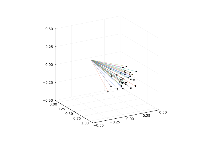
We have obtained a projection of the centroids of the stars onto a single sphere in the instrument coordinate system.
Conclusion
We managed to process the frame from the star sensor and translate the coordinates of the stars from a planar to a spherical coordinate system. To do this, we have tested several algorithms that have already been implemented in different libraries. The method of working on individual steps of the algorithm in separate code cells of the interactive script allowed us to conduct a number of computational experiments faster, displaying very complex and vivid illustrations, which accelerated the research process and made it possible to quickly find a satisfactory solution to the problem of filtering the image of the starry sky.
After the expensive prototyping stage, the algorithm can easily be translated into a more efficient form (for example, rewritten in C/C++) and placed in a model-oriented environment as a block from which code can be generated. Another direction of development of this work may be the development of a model of sensor errors, which is easy to implement with standard directional blocks on the Engee canvas.