Running the FMI model in Engee

Run FMU models in Julia environment to get simulation results and use them in further calculations.

Task description

The FMI (Functional Mockup Interface) standard involves packaging the model in an FMU (Functional Mockup Unit) file containing either a set of equations or code modelling the system (presumably supporting various programming languages that can be called in Engee: Python, Java, Fortran, C++, etc. including Julia).

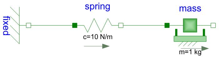
For an example, let's look at a spring and pendulum model built in Dymola. To run it we need the library FMI.jl and a set of training models, which are collected in the package FMIZoo.jl.

Pkg.add( ["FMI", "FMIZoo"] )

Let's connect the installed libraries:

using FMI
using FMIZoo

We are going to run a simulation of such a model:

The FMI.jl library allows you to run FMI/FMU models in several ways, and we will show two of them:

• through the command simulate
• through creating your own simulation loop and the command fmi2DoStep.

Create a time vector (set the start tStart, the end Stop of the simulation and the time step tStep):

tStart = 0.0
tStep = 0.1
tStop = 8.0
tSave = tStart:tStep:tStop

0.0:0.1:8.0

The simplest scenario for running an FMU model

Let's load the model SpringFrictionPendulum1D from the model package FMIZoo.jl.

fmu = loadFMU( "SpringFrictionPendulum1D", "Dymola", "2022x" )
info(fmu)

#################### Begin information for FMU ####################
	Model name:			SpringFrictionPendulum1D
	FMI-Version:			2.0
	GUID:				{2e178ad3-5e9b-48ec-a7b2-baa5669efc0c}
	Generation tool:		Dymola Version 2022x (64-bit), 2021-10-08
	Generation time:		2022-05-19T06:54:12Z
	Var. naming conv.:		structured
	Event indicators:		24
	Inputs:				0
	Outputs:			0
	States:				2
		33554432 ["mass.s"]
		33554433 ["mass.v", "mass.v_relfric"]
	Parameters:			12
		16777216 ["fricScale"]
		16777217 ["s0"]
		16777218 ["v0"]
		16777219 ["fixed.s0"]
		...
		16777223 ["mass.smin"]
		16777224 ["mass.v_small"]
		16777225 ["mass.L"]
		16777226 ["mass.m"]
		16777227 ["mass.fexp"]
	Supports Co-Simulation:		true
		Model identifier:	SpringFrictionPendulum1D
		Get/Set State:		true
		Serialize State:	true
		Dir. Derivatives:	true
		Var. com. steps:	true
		Input interpol.:	true
		Max order out. der.:	1
	Supports Model-Exchange:	true
		Model identifier:	SpringFrictionPendulum1D
		Get/Set State:		true
		Serialize State:	true
		Dir. Derivatives:	true
##################### End information for FMU #####################

Run the calculation of this model, specifying the start and end of the simulation time and the stored variable mass.s. Since there is friction in the model, the oscillations occur with decreasing amplitude, and after some time the load comes to rest.

simData = simulate(fmu, (tStart, tStop); recordValues=["mass.s"], saveat=tSave)
plot( simData )

After the calculation is finished, the FMU model must be unloaded from the memory and all time data must be deleted.

unloadFMU(fmu)

Creating your own simulation cycle

In a more complex case, such as when you need to link the work of several models, you can organise a computational loop in which the model takes steps in its phase space along some time vector.

Let's load the FMU model:

fmu = loadFMU("SpringFrictionPendulum1D", "Dymola", "2022x")

Model name:	SpringFrictionPendulum1D
Type:		1

The step function expects a specially prepared model (concrete implementation), which we will create using fmi2Instantiate. In this way many models can be initialised from one FMU file.

instanceFMU = fmi2Instantiate!(fmu)

FMU:            SpringFrictionPendulum1D
    InstanceName:   SpringFrictionPendulum1D
    Address:        Ptr{Nothing} @0x000000001d62f8c0
    State:          0
    Logging:        false
    FMU time:       -Inf
    FMU states:     nothing

In the next cell we perform the experiment setup (fmi2SetupExperiment), where we specify the start and end of the time interval for the simulation, then the model should be put into initialisation mode (fmi2EnterInitializationMode) and get its initial state after initialisation (fmi2ExitInitializationMode).

fmi2SetupExperiment(instanceFMU, tStart, tStop)

fmi2EnterInitializationMode(instanceFMU) # установить исходное состояние
fmi2ExitInitializationMode(instanceFMU)  # прочитать исходное состояние

0x00000000

Now we can run the model in the computational loop. The fixed step function fmi2DoStep tStep allows the computational steps of this model. If the model has input parameters or accepted data, they can be changed in the loop.

values = []

for t in tSave
    # выставить входные параметры модели, если требуется
    # ...

    fmi2DoStep(instanceFMU, tStep)
    
    # сохранить выходы модели
    value = fmi2GetReal(instanceFMU, "mass.s")
    push!(values, value)
end

plot(tSave, values)

At the end of the calculation we must free the memory and delete the intermediate files.

fmi2Terminate(instanceFMU)
fmi2FreeInstance!(instanceFMU)
unloadFMU(fmu)

[OK][CvodeStatistics][SpringFrictionPendulum1D]: Sundials CVode Statistics
    Stop time                                : 8.00 s
    Simulation time                          : 1.42 s
    Number of external steps                 : 80
    Number of internal steps                 : 191
    Number of non-linear iterations          : 263
    Number of non-linear convergence failures: 0
    Number of f function evaluations         : 291
    Number of g function evaluations         : 339
    Number of Jacobian-evaluations (direct)  : 7
    Maximum integration order                : 5
    Suggested tolerance scale factor         : 1.0
    Grouping used                            : no

Conclusion

We ran a simple FMU model using a single command, and figured out how to organise a computational loop where we could update the input parameters of the model and make operational decisions based on the output data.