Using MATLAB code in the Engee environment
This example demonstrates how to call MATLAB functions in Engee, as well as their application and comparison with environment functions.
Building curves in Engee:
Enabling the backend method for displaying graphics:
Pkg.add(["Statistics"])
using Plots
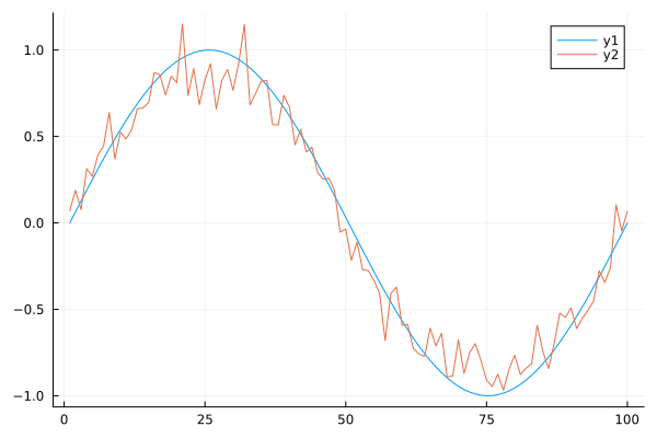
We generate two signals:
A = sin.(range(0, 2pi, length=100)')' # the sine wave
B = @. sin(A) + 0.1 * randn() # noisy sine wave
C = 1:1:100;
We display two signals on the graph:
plot(C,A)
plot!(C,B)
We calculate the correlation between the two signals by first connecting the library of statistical functions.:
using Statistics
engee_cor = cor(A,B)
Calling MATLAB code from Engee
From Julia, you can call any command or function MATLAB, which will return the result.
Connect the MATLAB interface:
using MATLAB
Loading signal data from Engee into the MATLAB core:
D = hcat(A,B)
A = D[:,1];
B = D[:,2];
mat"""
A = $A;
B = $B;
R = corrcoef(A,B);
"""
Calculating the correlation between two signals using the MATLAB kernel function:
matlab_cor = mat"R; R()"
Comparison of results and calculation of the absolute error of using methods from MATLAB and Engee:
difference = abs(engee_cor[1,1] - matlab_cor[1,2])
println("Engee Correlation: ", engee_cor[1,1], '\n', "Matlab Correlation: ", matlab_cor[1,2], '\n', "Absolute error: ", difference)
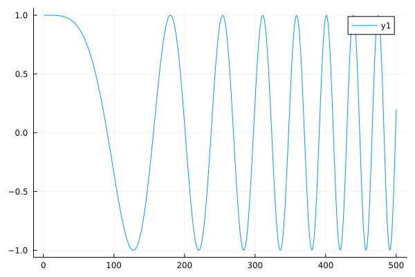
Calling a sinusoid with increasing frequency from MATLAB:
chirp = mat"chirp = dsp.Chirp('InitialFrequency', 0,'SamplesPerFrame', 500); chirp()"
plot(chirp)
Building a magic square:
mat"magic(3)"
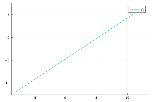
The simplest arithmetic operations:
x = range(-10.0, stop=10.0, length=50)
y = range(2.0, stop=3.0, length=50)

mat"""
    $u = $x + $y
    $v = $x - $y
"""

plot(u,v)
Calling MATLAB files from Engee
The path to the folder opened in the file manager:
mat"cd $(@__DIR__)"
Running the m script:
mat"file"
mat"run('file.m')"
mat"""run("file.m")"""
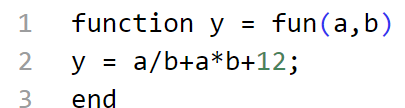
Launching MATLAB-functions:
.png)
mat"fun(10,9)"
x = 12;
y = 13.12;

z = mat"fun($x,$y)"

z/10
Viewing the workspace MATLAB:
mat"whos"
Cleaning up the workspace MATLAB:
mat"clear"
mat"whos"
Conclusion:
This example demonstrates the use of MATLAB functions in the Engee environment, their joint use, as well as the numerical difference between the methods used.