Python neural networks and their integration with Engee models

In this demonstration, we will look at an example of training neural networks using the sklearn package.

To work with neural networks using Python in Engee, the PyCall package and Python call commands in Engee are used.

First, let's install the sklearn and PyPlot libraries in Engee.

Pkg.add(["PyPlot"])

using Pkg
Pkg.add("ScikitLearn")
Pkg.add("PyPlot")

using PyPlot

# Импорт необходимых модулей из Python
@pyimport sklearn.neural_network as nn
@pyimport sklearn.tree as tree
@pyimport numpy as np

   Resolving package versions...
  No Changes to `/user/.project/Project.toml`
  No Changes to `/user/.project/Manifest.toml`
   Resolving package versions...
  No Changes to `/user/.project/Project.toml`
  No Changes to `/user/.project/Manifest.toml`

Generating training data from a model in Engee

This model generates a vector of two sinusoidal values that represent a single signal for the classifier. Based on the determination of the amplitude fluctuation of the output signal, the class labels are set. The figure below shows the top level of the model.

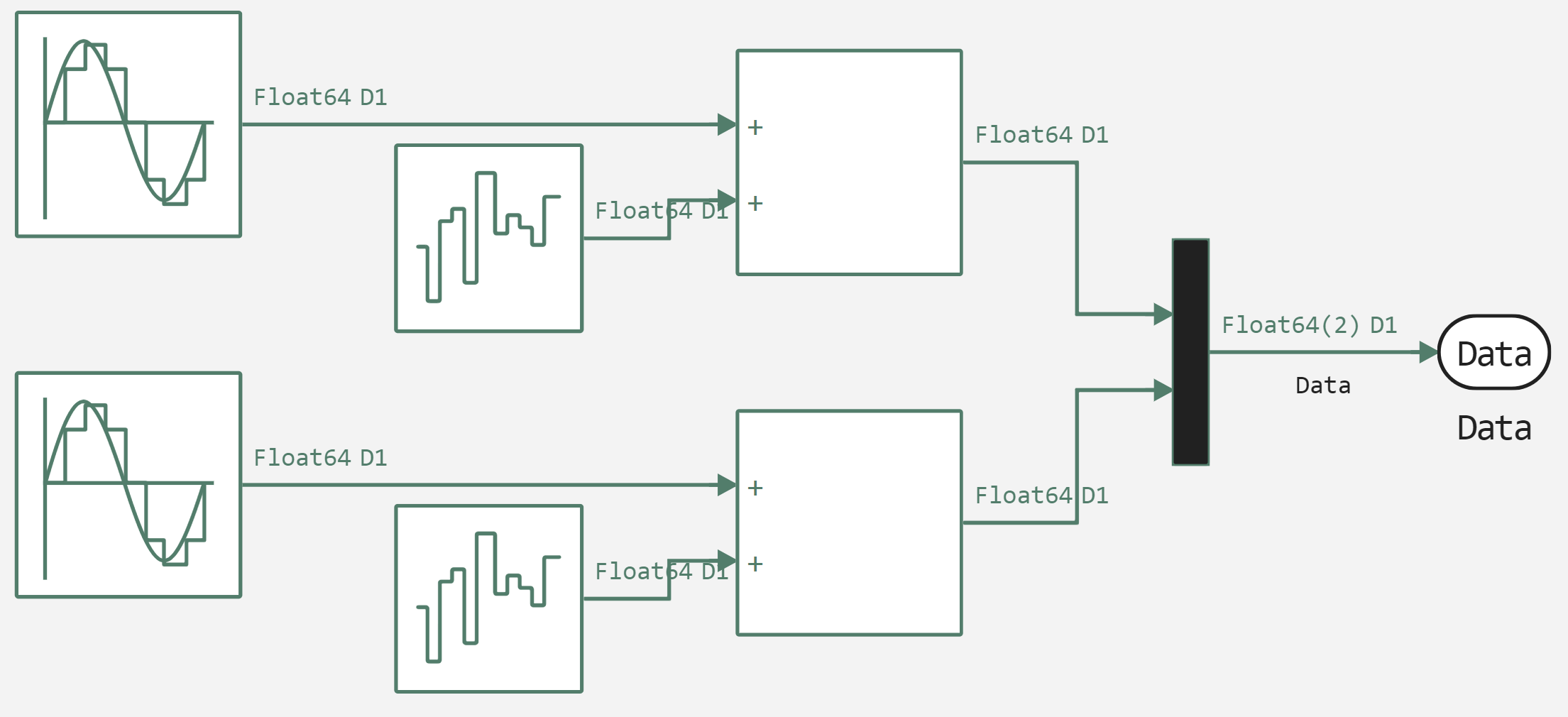
In the figure below, you can see the data generation process.

The following shows the formation of the class label over three ranges:

1. less than -0.7;
2. greater than -0.7 and less than 0.7;
3. greater than 0.7.

Let's move on to data generation by connecting the auxiliary function to run the model, run the model and see what data has been logged into simout.

 function run_model(name_model)
    Path = (@__DIR__) * "/" * name_model * ".engee"

    if name_model in [m.name for m in engee.get_all_models()] # Проверка условия загрузки модели в ядро
        model = engee.open( name_model ) # Открыть модель
        model_output = engee.run( model, verbose=true ); # Запустить модель
    else
        model = engee.load( Path, force=true ) # Загрузить модель
        model_output = engee.run( model, verbose=true ); # Запустить модель
        engee.close( name_model, force=true ); # Закрыть модель
    end

    return model_output
end

run_model("PyDataGen")
sleep(5)
collect(simout)

Building...
Progress 100%

2-element Vector{WorkspaceArray}:
 WorkspaceArray("PyDataGen/target")
 WorkspaceArray("PyDataGen/Data")

Next, we will unload the data from simout and convert it to numpy format for further feeding into Python neural networks.

target = simout["PyDataGen/target"];
target = collect(target);
target = np.array(target.value); 

Data = simout["PyDataGen/Data"];
Data = collect(Data);
Data = np.array(Data.value); 

Multilayer perseptron

The first network, a classifier, that we consider in this demonstration is a multilayer perseptron network for predicting data group membership based on oscillation amplitude.

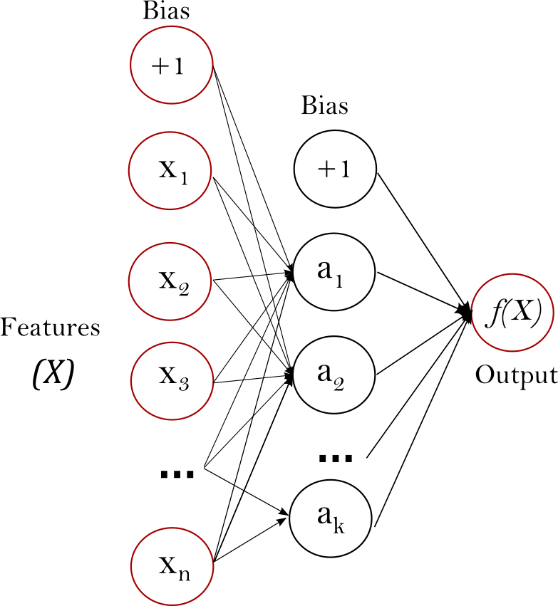
A multilayer perseptron (MLP) is a model of a feed-forward artificial neural network that maps sets of input data to a set of corresponding output data. MLP consists of several layers, each layer is fully connected to the next. The nodes of the layers are neurons with nonlinear activation functions, except for the nodes of the input layer. There may be one or more nonlinear hidden layers between the input layer and the output layer.

The figure below shows an MLP with one hidden layer with scalar output.

Let's move on to initialising and training the neural network in Python. There are several parameters to configure MLP:

1. hidden_layer_sizes - the size of the hidden layer;
2. max_iter - the maximum allowed number of training iterations;
3. alpha - training step;
4. solver - solver that defines the algorithm for optimising the weights on the nodes;
5. verbose - specifies whether to output additional information;
6. random_state - setting to control random values;
7. learning_rate_init - learning rate.

clf = nn.MLPClassifier(hidden_layer_sizes=(100,), max_iter=10, alpha=1e-4, solver="sgd", verbose=1, random_state=1, learning_rate_init=.1)
clf[:fit](Data, target)

Iteration 1, loss = 0.46645339
Iteration 2, loss = 0.19354594
Iteration 3, loss = 0.16433983
Iteration 4, loss = 0.11406597
Iteration 5, loss = 0.08521321
Iteration 6, loss = 0.07406608
Iteration 7, loss = 0.06680852
Iteration 8, loss = 0.06030754
Iteration 9, loss = 0.05545317
Iteration 10, loss = 0.05337739

/home/engee/.local/lib/python3.10/site-packages/sklearn/neural_network/_multilayer_perceptron.py:691: ConvergenceWarning: Stochastic Optimizer: Maximum iterations (10) reached and the optimization hasn't converged yet.
  warnings.warn(

MLPClassifier(learning_rate_init=0.1, max_iter=10, random_state=1, solver='sgd',
              verbose=1)

In a Jupyter environment, please rerun this cell to show the HTML representation or trust the notebook.
On GitHub, the HTML representation is unable to render, please try loading this page with nbviewer.org.

As we can see from the warning, the maximum number of iterations was reached and the optimisation did not converge. Hence, we need to increase the number of iterations. Let's repeat the initialisation and training of the neural network in Python with new network parameters.

clf = nn.MLPClassifier(hidden_layer_sizes=(100,), max_iter=140, alpha=1e-4, solver="sgd", verbose=1, random_state=1, learning_rate_init=.1)
clf[:fit](Data, target)

Iteration 1, loss = 0.46645339
Iteration 2, loss = 0.19354594
Iteration 3, loss = 0.16433983
Iteration 4, loss = 0.11406597
Iteration 5, loss = 0.08521321
Iteration 6, loss = 0.07406608
Iteration 7, loss = 0.06680852
Iteration 8, loss = 0.06030754
Iteration 9, loss = 0.05545317
Iteration 10, loss = 0.05337739
Iteration 11, loss = 0.07365467
Iteration 12, loss = 0.07634969
Iteration 13, loss = 0.05300259
Iteration 14, loss = 0.04155833
Iteration 15, loss = 0.04288358
Iteration 16, loss = 0.03979422
Iteration 17, loss = 0.03755778
Iteration 18, loss = 0.03600333
Iteration 19, loss = 0.03487557
Iteration 20, loss = 0.05186823
Iteration 21, loss = 0.05309877
Iteration 22, loss = 0.08833225
Iteration 23, loss = 0.19890236
Iteration 24, loss = 0.15260708
Iteration 25, loss = 0.07354444
Iteration 26, loss = 0.03785151
Iteration 27, loss = 0.03273216
Iteration 28, loss = 0.03582461
Iteration 29, loss = 0.03376020
Iteration 30, loss = 0.03097535
Iteration 31, loss = 0.02980889
Iteration 32, loss = 0.02932327
Iteration 33, loss = 0.02890707
Iteration 34, loss = 0.05155597
Iteration 35, loss = 0.07490897
Iteration 36, loss = 0.06002730
Iteration 37, loss = 0.03951461
Iteration 38, loss = 0.02728444
Iteration 39, loss = 0.02642886
Iteration 40, loss = 0.02672270
Iteration 41, loss = 0.07997178
Iteration 42, loss = 0.13905469
Iteration 43, loss = 0.11449981
Iteration 44, loss = 0.06326721
Iteration 45, loss = 0.03555334
Iteration 46, loss = 0.02623475
Iteration 47, loss = 0.02673499
Iteration 48, loss = 0.02717837
Iteration 49, loss = 0.02605130
Iteration 50, loss = 0.02468263
Iteration 51, loss = 0.02407942
Iteration 52, loss = 0.02379672
Iteration 53, loss = 0.02340889
Iteration 54, loss = 0.02314419
Iteration 55, loss = 0.02285639
Iteration 56, loss = 0.02264344
Iteration 57, loss = 0.02245725
Iteration 58, loss = 0.02222866
Iteration 59, loss = 0.02194008
Iteration 60, loss = 0.02181772
Iteration 61, loss = 0.02159413
Iteration 62, loss = 0.02155721
Iteration 63, loss = 0.02121266
Iteration 64, loss = 0.02106637
Iteration 65, loss = 0.02089924
Iteration 66, loss = 0.02104070
Iteration 67, loss = 0.02061003
Iteration 68, loss = 0.02046612
Iteration 69, loss = 0.02037115
Iteration 70, loss = 0.02015393
Iteration 71, loss = 0.02016866
Iteration 72, loss = 0.01998808
Iteration 73, loss = 0.01971004
Iteration 74, loss = 0.01963106
Iteration 75, loss = 0.01956479
Iteration 76, loss = 0.01939806
Iteration 77, loss = 0.01932444
Iteration 78, loss = 0.01912949
Iteration 79, loss = 0.01914763
Iteration 80, loss = 0.01893173
Iteration 81, loss = 0.01883002
Iteration 82, loss = 0.01876786
Iteration 83, loss = 0.01865177
Iteration 84, loss = 0.01856435
Iteration 85, loss = 0.01855969
Iteration 86, loss = 0.01848173
Iteration 87, loss = 0.01967259
Iteration 88, loss = 0.02043949
Iteration 89, loss = 0.01905147
Iteration 90, loss = 0.01793201
Iteration 91, loss = 0.01791697
Iteration 92, loss = 0.01804524
Iteration 93, loss = 0.01785849
Iteration 94, loss = 0.01777583
Iteration 95, loss = 0.02128908
Iteration 96, loss = 0.02461192
Iteration 97, loss = 0.01987342
Iteration 98, loss = 0.01746790
Iteration 99, loss = 0.03887814
Iteration 100, loss = 0.05479366
Iteration 101, loss = 0.03715838
Iteration 102, loss = 0.02011692
Iteration 103, loss = 0.01672488
Iteration 104, loss = 0.01805092
Iteration 105, loss = 0.01786109
Iteration 106, loss = 0.01683251
Iteration 107, loss = 0.01659169
Iteration 108, loss = 0.01669758
Iteration 109, loss = 0.01644202
Iteration 110, loss = 0.01629080
Iteration 111, loss = 0.01624752
Iteration 112, loss = 0.01626354
Iteration 113, loss = 0.01621645
Iteration 114, loss = 0.01615170
Iteration 115, loss = 0.01607716
Iteration 116, loss = 0.01619078
Iteration 117, loss = 0.01606433
Iteration 118, loss = 0.01595880
Iteration 119, loss = 0.01585314
Iteration 120, loss = 0.01576544
Iteration 121, loss = 0.01571510
Iteration 122, loss = 0.01566724
Iteration 123, loss = 0.01559469
Iteration 124, loss = 0.01556307
Iteration 125, loss = 0.01554502
Iteration 126, loss = 0.01544643
Iteration 127, loss = 0.01543122
Iteration 128, loss = 0.01556698
Iteration 129, loss = 0.01535017
Iteration 130, loss = 0.01533538
Training loss did not improve more than tol=0.000100 for 10 consecutive epochs. Stopping.

MLPClassifier(learning_rate_init=0.1, max_iter=140, random_state=1,
              solver='sgd', verbose=1)

In a Jupyter environment, please rerun this cell to show the HTML representation or trust the notebook.
On GitHub, the HTML representation is unable to render, please try loading this page with nbviewer.org.

Now let us evaluate the quality of the model. As we can see, the neural network has high guessing accuracy.

accuracy = clf[:score](Data, target)
println("Точность: $accuracy")

Точность: 0.998001998001998

Decision tree

Let's consider an example of code for training a neural network with a decision tree structure. This is a non-parametric learning method with a teacher, used for classification and regression.

This method requires creating a model that predicts the value of a target variable by learning simple decision rules inferred from data features.

The tree can be viewed as a piecewise constant approximation. We start by declaring and training the decision tree.

dt_clf = tree.DecisionTreeClassifier()
dt_clf.fit(Data, target)

DecisionTreeClassifier()

In a Jupyter environment, please rerun this cell to show the HTML representation or trust the notebook.
On GitHub, the HTML representation is unable to render, please try loading this page with nbviewer.org.

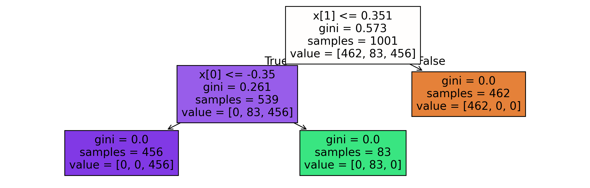
Let's construct a graph of the decision tree and increase the pixel size and density to make the graph more visual.

plt.figure(figsize=(13, 4), dpi=200)
tree.plot_tree(dt_clf, filled=true)

5-element Vector{PyObject}:
 PyObject Text(0.6, 0.8333333333333334, 'x[1] <= 0.351\ngini = 0.574\nsamples = 1001\nvalue = [461, 85, 455]')
 PyObject Text(0.4, 0.5, 'x[0] <= -0.352\ngini = 0.265\nsamples = 540\nvalue = [0, 85, 455]')
 PyObject Text(0.2, 0.16666666666666666, 'gini = 0.0\nsamples = 455\nvalue = [0, 0, 455]')
 PyObject Text(0.6, 0.16666666666666666, 'gini = 0.0\nsamples = 85\nvalue = [0, 85, 0]')
 PyObject Text(0.8, 0.5, 'gini = 0.0\nsamples = 461\nvalue = [461, 0, 0]')

Create a new graph to display the result of the neural network.

plt.figure(figsize=(18, 6), dpi=80)  # увеличим размер и плотность пикселей
plt.scatter(Data[:, 1], Data[:, 2], c=target, cmap=plt.cm.Paired, edgecolors="k")
plt.title("Neural Network")

PyObject Text(0.5, 1.0, 'Neural Network')

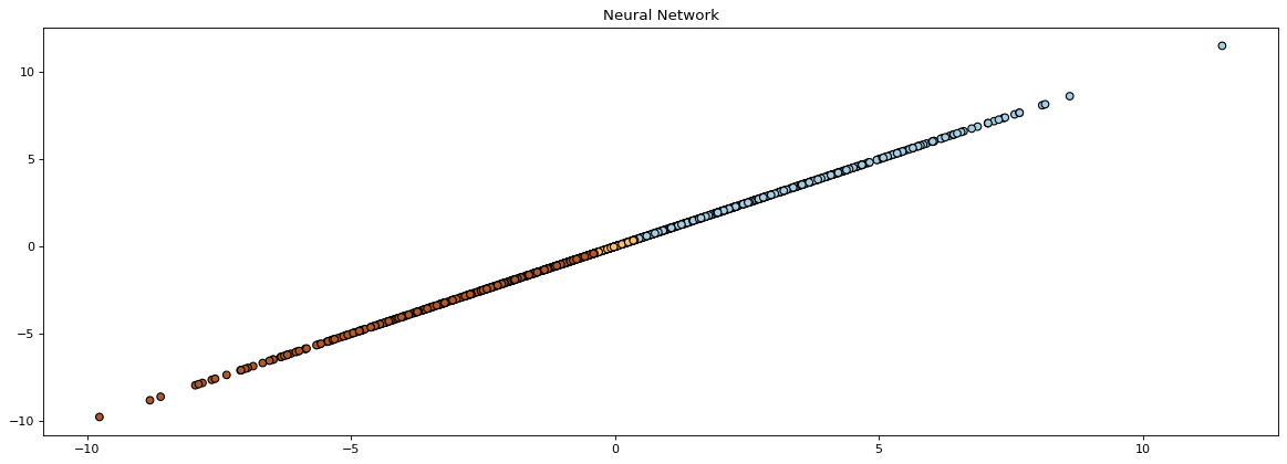
As we can see from the resulting graph, all the values we generated were distributed into three separate groups based on the sum of input data.

Conclusion

We have shown with concrete examples the options for integrating neural networks into Engee, as well as the possibilities of combining model-oriented design and Python functionality.

Blocks used in example

• Band-Limited White Noise
• Bit to Integer Converter
• Mux
• Sine Wave Function
• Switch