Euler's method for modeling the motion of a spherical body in water
Modeling the motion of bodies in liquids is an important part of projects in various fields of science
and technology, including hydrodynamics, oceanography, and engineering mechanics. In this example, the application of the numerical Eulerian method for motion modeling is considered.
a spherical body in water.
This method allows you to take into account the influence of gravity, the density of the medium and body, as well
as the resistance of the liquid.
The explicit first-order Eulerian method is used to solve the problem.
This is one of the simplest methods of numerical integration of ordinary
differential equations (ODES), which allows approximating the solution of the ODE to
at each time step. The basic idea of the method is as follows: the current
value of a function is approximated through its derivative multiplied by a small
time interval.
Our goal was to develop a program in Julia and MATLAB that simulates
body movement and visualizes the results as graphs of changes in diving depth and body velocity over time.
We will also compare the speed of identical scripts in these two languages and analyze the syntactic differences.
Next, for comparison, we will describe the MATLAB and Julia code in separate functions with
the output of the results of measurements of the time spent on initialization, calculations in the loop
and the output of graphs.
using MATLAB
using Images

function test_MATLAB()
    mat"""
    tic
        rho_w = 1000; % Water density (kg/m3)
        rho = 800; % Body density (kg/m3)
        g = 9.81; % Acceleration of gravity (m/s^2)
        dt = 0.01; % Time step (s)
        T = 5; % Total simulation time (s)
        % Number of steps
        N = round(T / dt);
        % Arrays for storing results
        z = 0; % Initial depth (m)
        v = 0; % Initial velocity (m/s)
        time = 0; % Time
    T = toc;
    disp("Initialization time: " + string(T))
    tic
        % Modeling
        for n = 1:N-1
            time(n+1) = dt * n;
            z(n+1) = z(n) + v(n) * dt;
            v(n+1) = v(n) + g * (rho_w - rho) / rho * dt;
        end
    T = toc;
    disp("Cycle time: " + string(T))
    tic
        % Charting
        figure;
        % Depth of time
        subplot(1, 2, 1);
        plot(time, z);
        xlabel('Time (s)');
        ylabel('Depth (m)');
        grid on;
        % Speed of time
        subplot(1, 2, 2);
        plot(time, v);
        xlabel('Time (s)');
        ylabel('Speed (m/s)');
        grid on;
        saveas(gcf, 'mat_plot.png');
    T = toc;
    disp("Chart display time:" + string(T))
    """
end
import Pkg; Pkg.add("TickTock")
using TickTock

function test_Julia()
    start_time = time()
        rho_w = 1000.0  # Water density (kg/m3)
        rho = 800.0     # Body density (kg/m3)
        g = 9.81        # Acceleration of gravity (m/s2)
        dt = 0.01       # Time step (s)
        T = 5.0         # Total simulation time (s)
        N = floor(Int, T / dt) + 1 # Calculating the number of steps
        t = zeros(N)   # Time
        t[1] = 0.0     # Initial time
        z = zeros(N)      # Position (depth)
        z[1] = 0.0        # Starting position (m)
        v = zeros(N)      # Speed
        v[1] = 0.0        # Initial velocity (m/s)
    println("Initialization time: " * string(time() - start_time))
    start_time = time()
        # Motion simulation
        for n in 1:N-1
            t[n+1] = dt * n
            z[n+1] = z[n] + v[n] * dt
            v[n+1] = v[n] + g * (rho_w - rho) / rho * dt
        end
    println("Cycle time: " * string(time() - start_time))
    start_time = time()
        # Depth depends on time
        A = plot(t, z,
            xlabel="Time (s)",
            ylabel="Depth (m)")

        # Speed versus time
        B = plot(t, v,
            xlabel="Time (s)",
            ylabel="Speed (m/s)")

        fig = plot(A, B, legend=false)
        savefig(fig, "jl_plot.png")
    println("Chart display time:" * string(time() - start_time))
end
Let's look at the main differences between these implementations.
- Types of variables
MATLAB: dynamic typing, variable types are not
explicitly declared.
Julia: static typing, it is often required to specify
types of variables to improve performance.
- Indexing arrays
MATLAB: starts with one and is in parentheses ().
Julia: starts with one, but in square brackets [].
- Printing values
MATLAB: The disp function is used.
Julia: The println function is used.
- Comments
MATLAB: Single-line comments start with %.
Julia: One-line comments start with a #.
- Charts
MATLAB: The modification functions are broken down into many separate commands.
Julia: All changes to the charts are presented as plot parameters.
Now let's compare the speed of operation and the results of the algorithms.
test_MATLAB()
test_Julia()
Judging by the presented results, Julia is significantly
superior to MATLAB in terms of the speed of each
stage of the process. Below is a brief analysis of each stage.
-
Initialization in Julia is about 120 times faster.
-
Julia's cycle processing time is about 1300 times shorter.
-
The display of graphs in Julia is about 21 times faster.
# Uploading images
jl_plot = load("$(@__DIR__)/jl_plot.png")
mat_plot = load("$(@__DIR__)/mat_plot.png")

# Combining images
print("jl_plot, mat_plot")
hcat(jl_plot, imresize(mat_plot, size(jl_plot)))
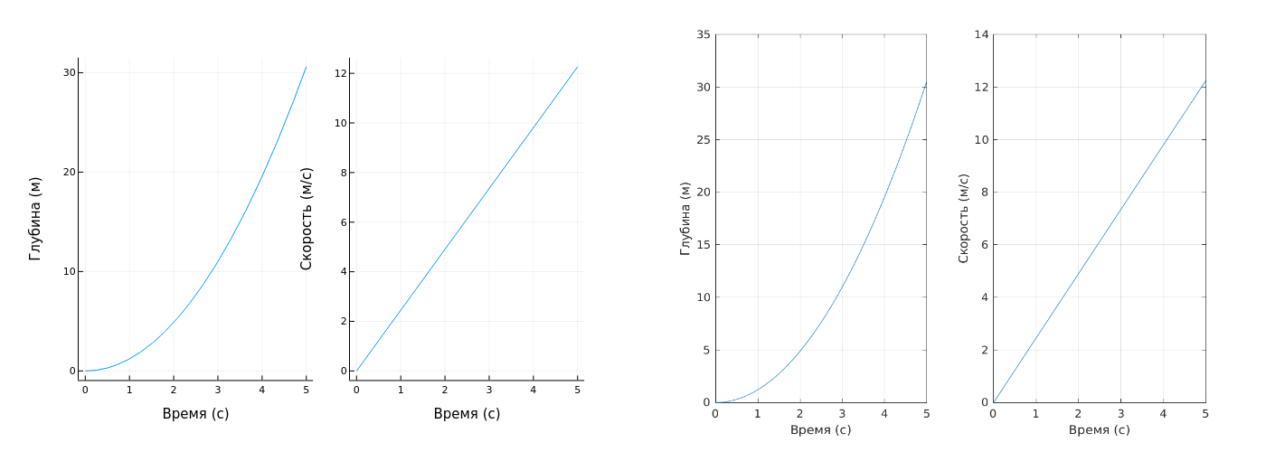
It can be seen that the graphs in both languages are of the same type. The same applies to the accuracy of calculations.
Conclusion
The syntax of languages is a matter of taste, a matter of purely subjective evaluation.
But the speed can be measured and assessed objectively. And it turns out that Julia works much faster at all.
The key stages of code execution are from initialization
to charting. These advantages can
may be due to stricter static typing,
JIT compilation and careful optimization of the language.
MATLAB, although it remains a powerful tool for scientific
calculations, is inferior to Julia in terms of speed, especially
when it comes to high-level computing tasks.,
where performance is critical.