Локальные двоичные структуры
В этой демонстрации показано, как можно использовать локальные двоичные структуры (LBP) в качестве очень эффективного классификатора текстур.
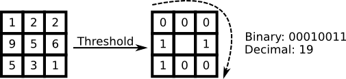
Оператор LBP маркирует пиксели изображения, сравнивая окрестность каждого пикселя с пороговым значением, и выдает результат в виде двоичного числа. В векторе признаков LBP значение соседним ячейкам на изображении в оттенках серого присваивается исходя из того, выше ли их значение порога (равного значению центральной ячейки) или ниже его.
Вычисление локальных двоичных структур:
-
Разделим исследуемое окно на ячейки (например, по
16x16пикселей). -
Сравним каждый пиксель в ячейке с каждым из его
8соседних пикселей (слева вверху, слева посередине, слева внизу, справа вверху и т. д.). Пиксели перебираются по кругу, то есть по часовой стрелке или против часовой стрелки. -
На предыдущем этапе количество рассматриваемых соседних пикселей можно изменить, изменив радиус окружности вокруг пикселя R и квантование углового пространства P.
-
Если значение центрального пикселя больше значения соседнего, записываем 0. В противном случае записываем 1. В результате получается 8-значное двоичное число (которое для удобства обычно преобразуется в десятичное).
-
Вычисляем для ячейки гистограмму (
histogram) частоты встречаемости каждого «числа» (то есть каждой комбинации пикселей, которые меньше и которые больше центра). Эту гистограмму можно рассматривать как 256-мерный вектор признаков. -
Дополнительно можно нормализовать
histogram. -
Объединяем гистограммы (возможно, нормализованные) всех ячеек. Получается вектор признаков для всего окна.
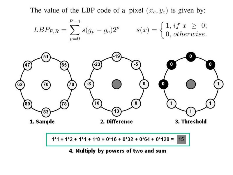 В приведенном выше примере показано вычисление LBP(P,R) для изображения в оттенках серого.
Результат шага 4 сохраняется в соответствующей ячейке итогового массива. Теперь вектор признаков можно обработать с помощью какого-либо алгоритма машинного обучения для классификации изображений. Такие классификаторы часто используются для распознавания лиц или анализа текстур.
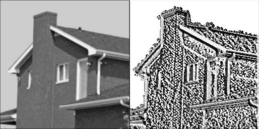
Теперь исследуем локальные двоичные структуры с помощью ImageFeatures.jl.
using ImageFeatures
using Images, TestImages
При построении дескриптора текстур LBP сначала необходимо получить изображение в оттенках серого. В этом примере мы используем изображение дома.
img = restrict(Gray.(testimage("house"))) # изображение дома размером 256*256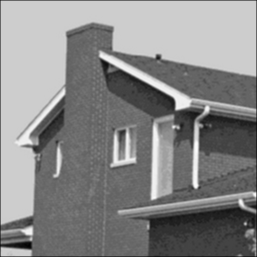
Для каждого пикселя на изображении в оттенках серого мы выбираем окрестность размером r вокруг центрального пикселя. Затем для этого центрального пикселя значение LBP вычисляется и сохраняется в выходном двухмерном массиве той же ширины и высоты, что и входное изображение.
Теперь вычислим выходную локальную двоичную структуру, используя API функции lbp, в котором необходимо указать method, points и radius. В ImageFeatures.jl есть несколько различных методов LBP, например lbp_original, lbp_uniform и lbp_rotation_invariant, но здесь мы используем оригинальный метод LBP.
-
points: количество рассматриваемых точек p в кругообразно симметричной окрестности (что устраняет необходимость в изучении квадратной окрестности). -
radius: радиус окружностиr, позволяющий учесть различные масштабы.
img_lbp = lbp(img, 8, 3, lbp_original); # используем оригинальную реализацию LBP
img_lbp = @. Gray.(img_lbp / 255.0) # преобразуем в нормализованное изображение в оттенках серого
edges, counts = build_histogram(img_lbp, 25, minval = 0, maxval = 1);
# plot(edges[1:end-1], counts[1:end-1]; title="LBP vs No. of Occurences", xlabel="Normalized LBP values", ylabel="Number of occurences")
(0.0:0.04:0.96, [0, 7531, 2661, 1087, 1613, 938, 1587, 1862, 657, 398 … 959, 372, 634, 1939, 1669, 764, 1559, 2026, 2821, 25345])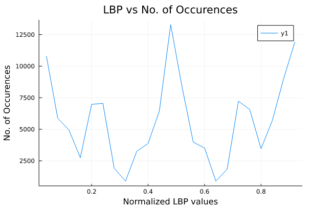
Используя эти ребра и числа, можно построить график, который даст представление о выходных локальных двоичных структурах. Локальные двоичные структуры дают представление об углах, плоскостях и краях на изображении. На этом графике пять пиков, которые можно классифицировать по следующим типам:
-
Угол: пики в окрестностях
x=0.2иx=0.7 -
Край: пик в центре в окрестности
x=0.5 -
Плоскость: пики возле
x=0.0иx=1.0
mosaicview(img, img_lbp; nrow = 1, rowmajor = true)