taylorwin
Taylor’s window.
| Library |
|
Arguments
Input arguments
# L — window length
+
scalar
Details
The window length specified as a positive integer.
If you specify L as a non-integer number, the function will round it to the nearest integer value.
|
| Data types |
|
# nbar — the number of side lobes of an almost constant level
+
4 (by default) | scalar
Details
The number of side lobes of an almost constant level adjacent to the main lobe is given as a positive integer. These side lobes are considered "almost constant level" because there is some attenuation in the transition region.
# sll — the maximum level of the side lobes relative to the peak of the main lobe
+
4 (by default) | scalar
Details
The maximum level of the side lobes relative to the peak of the main lobe is set as a valid negative scalar in dB. It creates side lobes with peaks on sll dB is below the peak of the main lobe.
Examples
Taylor’s Window
Details
We will generate a 64-point Taylor window with four side lobes that are almost constant in level and the peak level of the side lobe -35 dB is relative to the peak of the main lobe. Display the result using plot.
import EngeeDSP.Functions: taylorwin
using Plots
w = taylorwin(64, 4, -35)
plot(w,
     label = "Taylor Window",
     xlabel = "Sample Number",
     ylabel = "Amplitude",
     linewidth = 2,
     color = :blue,
     grid = true)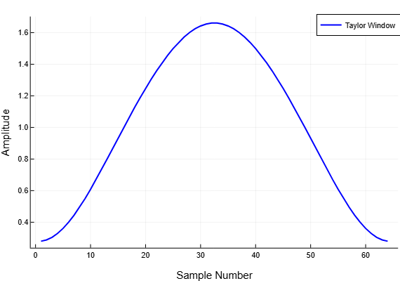
Algorithms
Taylor windows are similar to Chebyshev windows. The Chebyshev window has the narrowest possible main lobe for a given level of side lobes, but the Taylor window allows you to find a compromise between the width of the main lobe and the level of the side lobes. The Taylor distribution eliminates discontinuities at the edges of the radiation pattern, so the side lobes of the Taylor window decrease monotonically. Taylor window coefficients are not normalized. Taylor windows are commonly used in radar applications such as weighted synthetic aperture radars and antenna design.