kurtogram
Visualization of spectral kurtosis.
| Library |
|
Syntax
Function call
-
kgram,f,w,fc,wc,bw = kurtogram(x,out=:data)— returns a fast kurtogram signalxin the form of a matrixkgramand a set of parameters for subsequent bandpass filter design and spectral kurtosis analysis:To calculate the time values, the function
kurtogramuses a normalized frequency: evenly distributed frequency values in the range[0, π].
-
kgram,f,w,fc,wc,bw = kurtogram(___,level,out=:data)— returns a quick pictogram with the specified levellevel. This argument determines the resolution level of the window and the number of calculated values of the spectral kurtosis. It can be used with any input arguments from the previous syntax options.
-
kurtogram(___,out=:plot)— builds a graph showing the main optimization parameters. This syntax can be used with any input arguments from the previous options.
Arguments
Input arguments
# x is a time domain signal
+
vector
Details
A time domain signal defined as a vector. Function kurtogram calculates a fast pictogram of this signal.
# sampx — sampling frequency or sampling period of the signal
+
normalized frequency (by default) | scalar | vector | array
Details
The sampling frequency or sampling period of the signal, set to one of the following values:
-
A positive scalar is a frequency measured in Hz.;
-
Vector or array — time points corresponding to each element
x.
If sampx it is a vector, the samples may be uneven, but the function pspectrum imposes the following restriction on the ratio of the median and average time intervals:
If sampx set to empty, the function kurtogram It uses a normalized frequency, that is, the frequency vector has evenly distributed values in the range .
#
level —
maximum
courtogram level
scalar
Details
The maximum level of the courtogram, set as a positive integer. This argument determines the number of calculated values of the spectral kurtosis and the size of the windows used by the function. kurtogram, and hence the frequency resolution.
As the frequency resolution increases, the time resolution decreases. If any of these resolutions turn out to be too low, the estimate of the spectral kurtosis will be inaccurate. When choosing level The impact on both types of resolution must be considered.
Input arguments «name-value»
# out — type of output data
+
:plot (by default) | :data | :all
Details
Type of output data:
-
:plot— the function returns a graph; -
:data— the function returns data; -
:all— the function returns data and a graph.
Output arguments
# kgram — fast kurtogram
+
the matrix
Details
A fast kurtogram, returned as a matrix, the dimensions of which are determined by the argument level. The matrix contains 2 * level lines and 3 * 2level columns. Each row contains the results of calculating the spectral kurtosis for all elements of the frequency vector. f and for the window size determined by the row position relative to the following sequence:
where is the equivalent window size for the level compose the countdown.
# fc is the frequency of the maximum value of the spectral kurtosis
+
scalar
Details
The frequency of the maximum value of the spectral kurtosis in kgram returned as a scalar:
Meaning fc It can be used as the center frequency for an optimal bandpass filter that maximizes the envelope kurtosis of the filtered signal. Maximizing the envelope kurtosis makes it easier to identify the resulting impulse component as an informative feature.
# wc is the window size of the maximum spectral kurtosis value
+
scalar
Details
The size of the window of the maximum value of the spectral kurtosis in kgram, returned as a scalar in counts.
Meaning wc can be used as the optimal window size for the function pkurtosis. For an example, see Plotting the spectral kurtosis with a given window size.
# bw — recommended bandwidth for optimal bandpass filter
+
scalar
Details
Recommended bandwidth for an optimal bandpass filter, returned as a scalar:
Examples
Calculation of a nonstationary signal pictogram
Details
Let’s calculate the frequency range of the non-stationary signal, compare the different values of the maximum frequency level of the frequency range and analyze the frequency range with the normalized frequency. The obtained parameters can be used to determine the parameters of the filter used in signal preprocessing in order to improve transient detection.
Let’s create a chirp signal with white Gaussian noise.
fs = 1000
t = collect(0:1/fs:10)
f1 = 300
f2 = 400
xc = EngeeDSP.Functions.chirp(t, f1, 10, f2)
x = xc .+ randn(length(t))
Let’s build a kurtogram using the sampling frequency fs.
import EngeeDSP.Functions: kurtogram

kurtogram(x, fs)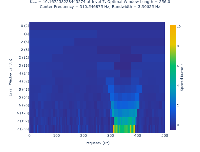
The kurtogram shows the kurtosis values for different window sizes and frequency ranges. A high kurtosis value indicates a pronounced nonstationarity or deviation from the Gaussian distribution. The maximum kurtosis value is indicated above the graph, as well as the corresponding window size and center frequency. The bandwidth depends on the size of the window.
Let’s explore the impact of reducing the maximum level to 5.
level = 5
kurtogram(x, fs, level)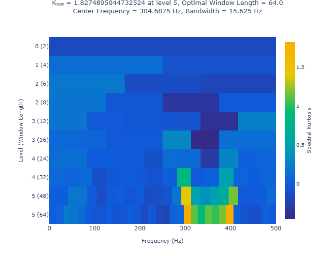
The decrease in resolution becomes obvious and leads to a decrease in the peak kurtosis value and a shift in the center frequency.
Now we will construct a kurtogram without specifying the sampling frequency or period.
kurtogram(x)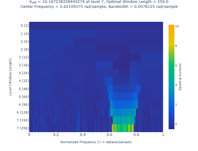
In this case, the courtogram is displayed with a normalized frequency.
The parameters above the graph allow you to select a band-pass filter for data preprocessing and improve the selection of the non-stationary component. Function kurtogram It can also return these parameters to use them directly in filtering functions or in spectral kurtosis analysis.
kgram, f, w, fc, wc, bw = kurtogram(x, out = :data)
println("wc = ", wc,
        "\nfc = ", fc,
        "\nbw = ", bw)
wc = 256.0
fc = 1.9512235621905356
bw = 0.02454369260617026Meaning wc corresponds to the optimal window size of the first graph, and fc and bw — its central frequency and bandwidth after the transition to the normalized frequency. Variable kgram it is a matrix of a kurtogram, and f and w — corresponding vectors of frequencies and window sizes.
Plotting the spectral kurtosis with a given window size
Details
Function pkurtosis uses the window size (time resolution) determined by the function pspectrum by default. You can set your own window size. In this example, we will determine the optimal window size using the function kurtogram and we use it when calculating the spectral kurtosis.
Let’s create a chirp signal with white Gaussian noise.
fs = 1000
t = collect(0:1/fs:10)
f1 = 300
f2 = 400
x = EngeeDSP.Functions.chirp(t, f1, 10, f2) .+ randn(length(t))
Let’s plot the spectral kurtosis with the default window size.
import EngeeDSP.Functions: pkurtosis

pkurtosis(x, fs)
plot!(title = "Spectral Kurtosis with Default Window Size", legend = (0.1, 0.93))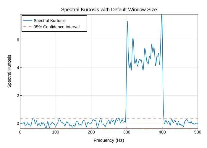
Let’s calculate the optimal window size using the function kurtogram.
import EngeeDSP.Functions: kurtogram

kurtogram(x, fs, out = :plot)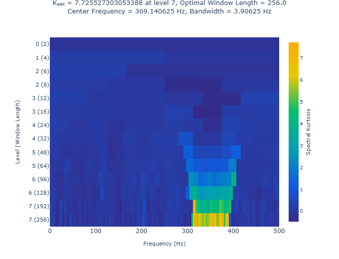
The kurtogram shows the chirp signal component in the range from 300 before 400 Hz and shows that the optimal window size is 256 counts. Passing this value in a variable w0 functions pkurtosis.
w0 = 256
pkurtosis(x, fs, w0)
plot!(title = "Spectral Kurtosis with Optimum Window Size of 256", legend = (0.1, 0.93))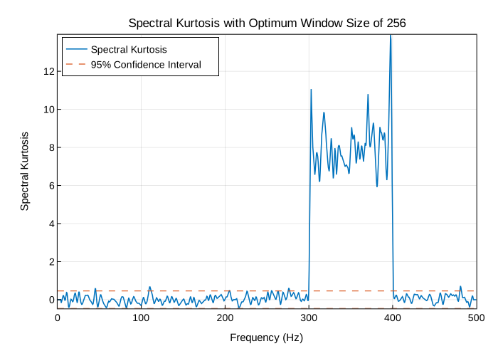
The main surge is characterized by higher kurtosis values. This improves the distinctness of the stationary and non-stationary components and facilitates the identification of the non-stationary component as an informative feature.
Additional Info
Courtogram
Details
Function kurtogram provides data for spectral kurtosis analysis. It calculates the spectral kurtosis for several window sizes using a fast graph algorithm. In addition to the icon itself and the corresponding vectors of frequencies and window sizes, the function returns the optimal window size and other filter settings. The calculation results can also be displayed on a graph.
The fast graph algorithm uses bandpass filtering and a simplified calculation scheme to approximate the spectral kurtosis for each window size and each frequency. More accurate algorithms use the short-term Fourier transform. In addition, compared with the full graph algorithm, this method reduces the number of iterations required to cover the plane. «frequency — window size» [1].