pkurtosis
The spectral kurtosis of the signal or spectrogram.
| Library |
|
Syntax
Function call
-
sk,fout,thresh = pkurtosis(x,out=:data)— returns the spectral kurtosis of the signalxin the form of a vectorsk, as well as the frequency vectorfout. To calculate the time parameters, the functionpkurtosisuses a normalized frequency: evenly distributed frequency values ranging from0beforeπrad/countdown. The spectrogram of the signal is calculated usingpspectrumwith default window size and overlapping windows80%.
-
sk,fout,thresh = pkurtosis(___,"ConfidenceLevel",p,out=:data)— also returns the threshold value of the spectral kurtosisthreshfor the level of trustp. The threshold defines the boundaries of the region in which the values of the spectral kurtosis correspond to a stationary Gaussian signal at the selected confidence level. The confidence level allows you to adjust the sensitivity of the threshold values of the spectral kurtosis to deviations from the Gaussian distribution or to the detection of non-stationary components of the signal.
-
pkurtosis(___)— plots the spectral kurtosis with an indication of the confidence level and thresholds. This syntax can be used with any input arguments from the previous options.
Arguments
Input arguments
# x is a time domain signal
+
vector
Details
A time domain signal defined as a vector. Function pkurtosis calculates the spectral kurtosis of this signal.
# sampx is the sampling frequency or sampling period of the signal
+
normalized frequency (by default) | scalar | vector | array
Details
The sampling frequency or sampling period of the signal, set to one of the following values:
-
A positive scalar is a frequency measured in Hz.;
-
Vector or array — time points corresponding to each element
x.
If sampx it is a vector, the samples may be uneven, but the function pspectrum imposes the following restriction on the ratio of the median and average time intervals:
If sampx set to empty, the function pkurtosis It uses a normalized frequency, that is, the frequency vector has evenly distributed values in the range .
# window — temporary window resolution
+
scalar
Details
The time resolution of the window, set as a positive scalar in counts. It is used in the internal calculation of the spectrogram using the function pspectrum. Argument window It is required when submitting an existing spectrogram to the input and is optional in other syntax variants. The optimal window size can be determined using the function kurtogram. By default pspectrum uses overlapping windows 80%.
# s is a spectrogram or a signal power spectrogram
+
the matrix | vector
Details
A spectrogram or signal power spectrum, defined as a matrix for a spectrogram or a column vector for a spectrum.
-
If
scontains complex values, the functionpkurtosisinterprets it as a short-term Fourier transform (FFT) of the original signal (spectrogram). -
If
scontains real values, the functionpkurtosisinterprets it as the square of the KVPF modulus of the original signal (power spectrogram). Each elementsmust be non-negative.
If the argument is s set, function pkurtosis uses it instead of calculating its own spectrogram or power spectrogram. For an example, see Plotting the spectral kurtosis according to a given spectrogram.
| Типы данных |
|
| Support for complex numbers |
Yes |
Input arguments «name-value»
Specify optional argument pairs as Name,Value, where Name — the name of the argument, and Value — the appropriate value. Type arguments «name-value» they should be placed after the other arguments, but the order of the pairs does not matter. You can specify multiple pairs «name-value».
Use commas to separate the name and value, and Name enclose it in quotation marks, or use an equal sign to separate the name and value, and Name specify it without quotation marks.
# ConfidenceLevel — the level of trust
+
0.95 (by default) | scalar
Details
The confidence level, set as a scalar p in the range of 0 before 1. It is used to determine whether the signal can be considered Gaussian and stationary. Meaning p affects the boundaries of the area defined by the threshold value thresh. Within this region, the value of the spectral kurtosis indicates the Gaussian and stationary nature of the signal. Thus, the confidence level allows you to adjust the detection sensitivity. Kurtosis values outside the region with probability they indicate a possible non-Gaussian or non-stationary behavior of the signal. For an example, see Plotting the spectral kurtosis of an unsteady signal at different confidence levels.
Output arguments
# sk — spectral kurtosis
+
vector
Details
Spectral kurtosis, returned as a vector of the type Float32 or Float64. Spectral kurtosis is a statistical quantity that takes small values where the data is stationary and has a Gaussian distribution, and high values where transients occur. Spectral kurtosis makes it possible to detect and localize non-stationary or non-Gaussian components that may be caused by malfunctions or deterioration of system characteristics. High kurtosis values indicate the presence of such signal components.
# threshold is the bandwidth of the spectral kurtosis for stationary Gaussian behavior
+
scalar
Details
The bandwidth of the spectral kurtosis for stationary Gaussian behavior, returned as a scalar. This value determines the thickness of the strip centered relative to the line. sk = 0, at a given level of trust ConfidenceLevel. Going outside the band bounded by the threshold thresh, indicates possible unsteady or non-Gaussian behavior. Argument ConfidenceLevel it directly affects the thickness of the strip and the sensitivity of the results. For an example, see Plotting the spectral kurtosis of an unsteady signal at different confidence levels.
Examples
Plotting the spectral kurtosis of an unsteady signal at different confidence levels
Details
Let’s plot the spectral kurtosis of a signal with linear frequency modulation and white noise to detect an unsteady non-Gaussian component. We investigate the impact of changes in the level of trust and the use of a normalized frequency.
Let’s create a chirp signal, add white Gaussian noise, and plot a graph.
import EngeeDSP.Functions: chirp

fs = 1000
t = collect(0:1/fs:10)
f1 = 300
f2 = 400

xc = chirp(t, f1, 10, f2)
x = xc .+ randn(length(t))

plot(t, x, title = "Chirp Signal with White Gaussian Noise")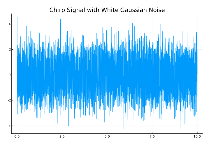
Let’s plot the spectral kurtosis of the signal.
import EngeeDSP.Functions: pkurtosis

pkurtosis(x, fs)
plot!(title = "Spectral Kurtosis of Chirp Signal with White Gaussian Noise",
      ylim = (-1, 9), legend = (0.64, 0.93))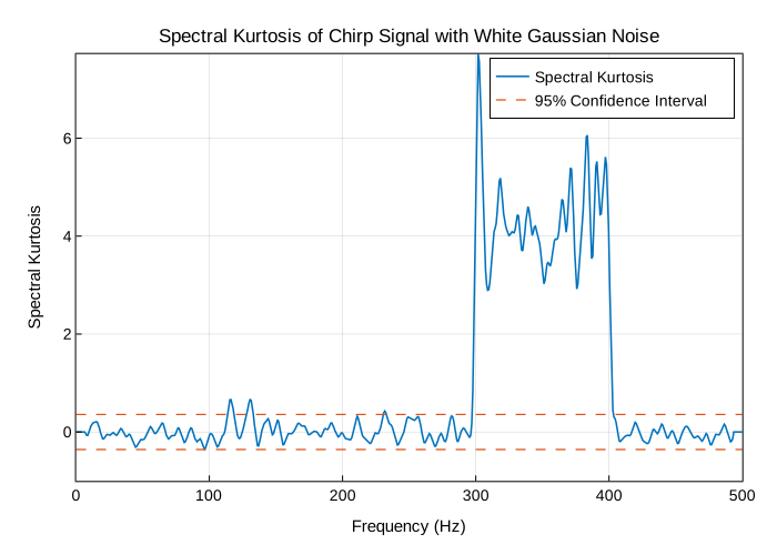
The graph shows a marked deviation in the range from 300 before 400 Hz, corresponding to the non-stationary component of the chirp signal. The area between the horizontal dashed lines corresponds to the zone of probable stationary and Gaussian behavior, determined by the confidence level 0.95. The kurtosis values falling within this zone are highly likely to characterize a stationary Gaussian process. Values outside of this zone are classified as non-stationary or non-Gaussian. A few small deviations below 300 Hz slightly exceeding the threshold value are false alarms: noise leads to exceeding the threshold for the stationary Gaussian component.
Let’s explore the impact of the trust level by changing its value from the default one. 0.95 on 0.85.
pkurtosis(x, fs, "ConfidenceLevel", 0.85)
plot!(title = "Spectral Kurtosis of Chirp Signal with Noise at Confidence Level of 0.85",
      ylim = (-1, 9), legend = (0.64, 0.93))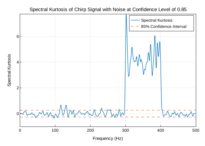
A lower confidence level provides increased sensitivity when detecting non-stationary or non-Gaussian frequency components. A decrease in the level of trust narrows the area limited by thresholds thresh. At the same time, the number and amplitude of low-level deviations (false alarms) increase. Choosing the confidence level allows you to find a balance between effective detection and limiting the number of false positives.
Let’s compare the width of the zone for both trust levels using the call option pkurtosis, which returns the corresponding value.
sk1, _, thresh95 = pkurtosis(x, out = :data)
sk2, _, thresh85 = pkurtosis(x, ConfidenceLevel = 0.85, out = :data)
thresh = [thresh95 thresh85]
1×2 Matrix{Float64}:
0.357839 0.262821Let’s plot the spectral kurtosis, excluding information about the sampling period, so that the function pkurtosis I used a normalized frequency.
pkurtosis(x, ConfidenceLevel = 0.85)
plot!(title = "Spectral Kurtosis using Normalized Frequency",
      ylim = (-1, Inf), legend = (0.64, 0.93))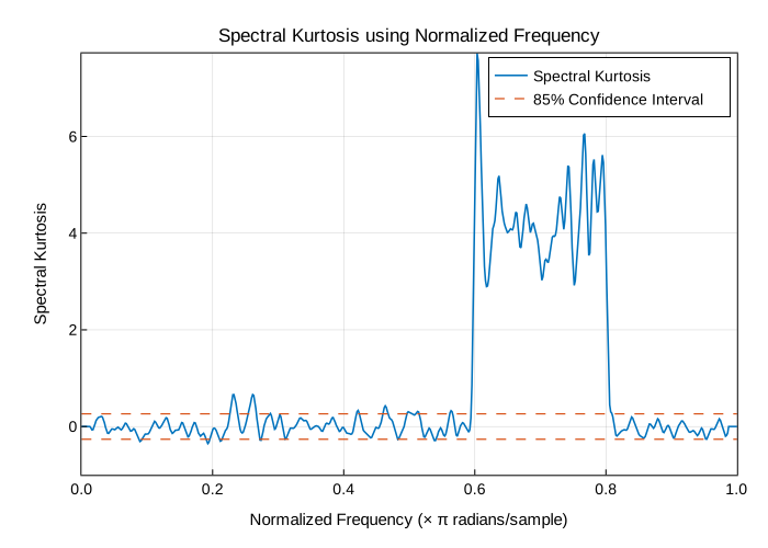
The frequency scale in Hz has been replaced by a normalized frequency scale from 0 before π rad/countdown.
Plotting the spectral kurtosis according to a given spectrogram
Details
When a signal is applied to the input, the function pkurtosis calculates the spectrogram using the function pspectrum using the default settings. To use your own settings, you can calculate the spectrogram in advance.
Let’s create a chirp signal containing white Gaussian noise.
import EngeeDSP.Functions: chirp

fs = 1000
t = collect(0:1/fs:10)
f1 = 300
f2 = 400

x = chirp(t, f1, 10, f2) .+ randn(length(t))
Calculate the spectrogram using the function spectrogram, setting the window size, overlap, and the number of FFT points. Then we use this spectrogram in pkurtosis.
import EngeeDSP.Functions: spectrogram, pkurtosis

window = 256
overlap = round(Int, window * 0.8)
nfft = 2 * window
s, f, t, p = spectrogram(x, window, overlap, nfft, fs = fs, out = :data)

pkurtosis(s, fs, f, window)
plot!(ylim = (-1, Inf), legend = (0.13, 0.93))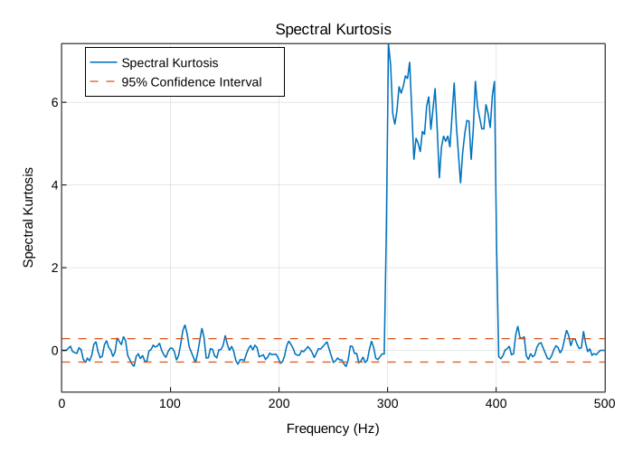
The amplitude of the spike is higher here — and, therefore, it is better distinguishable — than when using the default settings in the previous example.
Additional Info
Spectral kurtosis
Details
Spectral kurtosis is a statistical characteristic that makes it possible to detect and localize non—stationary or non-Gaussian processes in the frequency domain, characterized by:
-
small values at frequencies where only stationary Gaussian noise is present;
-
high positive values at frequencies where transients occur.
Spectral kurtosis is a powerful tool for detecting and isolating signals related to malfunctions of rotating mechanical systems. It allows you to identify signs or status indicators for fault detection and classification. During preprocessing for other methods, such as envelope analysis, the spectral kurtosis can provide important input data, such as optimal frequency band parameters [1], [2].
Spectral kurtosis The signal calculated on the basis of the short-term Fourier transform (FFT) :
where — window function. The spectral kurtosis is calculated using the formula
where — the time averaging operator.
If the signal is contains only stationary Gaussian noise, then at each frequency value It has an asymptotically normal distribution with zero mean and variance , where — the number of elements along the time axis in . Hence, the statistical threshold at the level of trust defined as
where — quantile function of the standard normal distribution.
It is important to note that the length of the window The QFT defines the frequency resolution , where — sampling rate. The window size should be less than the interval between the pulses of the transient process, but longer than the duration of these pulses themselves.
Literature
-
Antoni, J. «The Spectral Kurtosis: A Useful Tool for Characterising Non-Stationary Signals.» Mechanical Systems and Signal Processing. Vol. 20, Issue 2, 2006, pp. 282–307.
-
Antoni, J., and R. B. Randall. «The Spectral Kurtosis: Application to the Vibratory Surveillance and Diagnostics of Rotating Machines.» Mechanical Systems and Signal Processing. Vol. 20, Issue 2, 2006, pp. 308–331.