spectralCrest
Spectral crest for signals and spectrograms.
| Library |
|
Syntax
Function call
-
crest,spectralPeak,spectralMean = spectralCrest(x,f)— returns the spectral crest of the signalxover time, the peak of the spectrum and the spectral mean. Interpretationxthe function depends on the formf.
-
crest,spectralPeak,spectralMean = spectralCrest(x,f,Name,Value)— sets parameters using one or more name-value arguments.
-
spectralCrest(___,out=:plot)— plots the spectral ridge.-
If the input signal is in the time domain, the spectral crest graph is plotted as a function of time.
-
If the input signal is in the frequency domain, the spectral crest graph is plotted depending on the frame number.
-
Arguments
Input arguments
# f is the sampling frequency or frequency vector (Hz)
+
scalar | vector
Details
The sampling frequency or frequency vector in Hz, specified as a scalar or vector, respectively. Interpretation x the function depends on the form f:
-
If
f— scalar,xit is interpreted as a signal in the time domain, andf— as a sampling rate. In this casexmust be a real vector or a matrix. Ifxset as a matrix, the columns are interpreted as separate channels. -
If
f— vector,xit is interpreted as a signal in the frequency domain, andf— how are the frequencies in Hz corresponding to the stringsx. In this casexmust be a real array of size , where — the number of spectral values at the specified frequenciesf, — the number of individual spectra, and — the number of channels. -
Number of lines
x, , must be equal to the number of elementsf.
| Data types |
|
Name-value input arguments
Specify optional argument pairs as Name,Value, where Name — the name of the argument, and Value — the appropriate value. Name-value arguments should be placed after other arguments, but the order of the pairs does not matter.
Use commas to separate the name and value, and Name put it in quotation marks.
The following name-value arguments apply if x — a signal in the time domain. If x — the signal is in the frequency domain, arguments like "name-value" are ignored.
|
# Window — the window used in the time domain
+
rectwin(round(f*0.03)) (by default) | vector
Details
The window used in the time domain, defined as a real vector. The number of vector elements must be in the range [1,size(x,1)]. The number of vector elements must also be greater. OverlapLength.
| Data types |
|
# FFTLength — the number of elements in the DFT
+
numel(Window) (by default) | a positive integer scalar
Details
The number of elements used to calculate the DFT of window input samples, set as a positive integer scalar. If no argument is given, FFTLength by default, it is equal to the number of elements in Window.
| Data types |
|
# SpectrumType — spectrum type
+
"power" (by default) | "magnitude"
Details
The type of spectrum specified as "power" or "magnitude":
-
"power"— the spectral crest is calculated for a one-sided power spectrum; -
"magnitude"— the spectral crest is calculated for a one-sided amplitude spectrum.
| Data types |
|
# out — type of output data
+
:data (by default) | :plot
Details
Type of output data:
-
:data— the function returns data; -
:plot— the function returns a graph.
Examples
Spectral crest of the signal in the time domain
Details
Let’s create an FM signal with white Gaussian noise and calculate the crest using the default parameters.
import EngeeDSP.Functions: chirp, randn, spectralCrest

fs = 1000
t = (0:1/fs:10)
f1 = 300
f2 = 400
x = chirp(t, f1, 10, f2) + randn(length(t), 1)

crest = spectralCrest(x, fs)
Let’s plot the dependence of the spectral ridge on time.
spectralCrest(x, fs, out=:plot)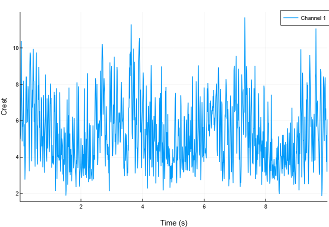
([4.987046327015055, 5.236871947723927, 7.544804457899835, 10.3772996669661, 7.705619466415934, 5.99985432220379, 4.868975479415114, 5.902444766668258, 5.6781203280701815, 6.523480840096338 … 7.803614225515488, 8.289150599849984, 8.382547366360493, 6.028262627692971, 6.683863065009292, 5.194224063455523, 3.7499682104979466, 5.218718311184415, 3.207068721139457, 6.082745967003252], [0.439680011925611, 0.601102975643176, 1.034484757673182, 1.3330997948299792, 0.8496287200130014, 0.4947671774843161, 0.43476209921716236, 0.5070692566692776, 0.6240111902833801, 0.8937070726200211 … 0.962580947281854, 1.2053879463201618, 1.4011032035761652, 0.8161989525511318, 0.716299380591645, 0.37571979028258434, 0.25389759893331165, 0.48721486174074174, 0.31362312100811496, 0.6811440879165471], [0.08816441298005284, 0.11478282868925793, 0.13711220263502233, 0.12846307205270513, 0.11026092369549412, 0.08246319842355515, 0.08929231643396737, 0.08590834420556587, 0.1098974932247451, 0.1369984973554123 … 0.1233506577163312, 0.14541754692476894, 0.16714527724577494, 0.1353953871886124, 0.10716847033290458, 0.072334151490691, 0.06770660034464596, 0.09335910326805238, 0.09779120694884458, 0.11197970318200254], Plot{Plots.PlotlyJSBackend() n=1})Spectral crest of the signal in the frequency domain
Details
Let’s create an LFM signal with white Gaussian noise, and then calculate the spectrogram using the function stft.
import EngeeDSP.Functions: chirp, randn, stft

fs = 1000
t = (0:1/fs:10)'
f1 = 300
f2 = 400
x = chirp(t, f1, 10, f2) + randn(size(t)...)

s, f = stft(x, fs, "FrequencyRange", "onesided")
s = abs.(s).^2
Calculate the crest of the spectrogram over time.
import EngeeDSP.Functions: spectralCrest

crest = spectralCrest(s, f)
Let’s plot the dependence of the spectral ridge on the frame number.
spectralCrest(s, f, out=:plot)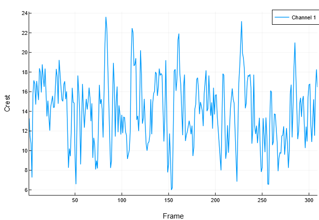
([13.278262719339581, 11.423943909400123, 10.704344652278133, 7.265409265608759, 15.671348771900583, 17.14664360019774, 16.805060471491807, 14.696328543184194, 17.09013028905847, 15.936360071580983 … 16.710312667671143, 16.761812477538534, 12.62023888820894, 10.886155724606253, 13.208164879678929, 15.219986950457587, 11.520098623729307, 16.272350151097733, 18.269299846830197, 16.45774860128549], [1038.875221526367, 1003.8420042054646, 878.9222908403066, 340.3639889446644, 1013.9709212810934, 1511.5917119138305, 1166.5576026614406, 845.4456363019548, 1122.2172446705913, 1132.3238949123497 … 1483.6967321132968, 1213.326351390993, 859.9980861071526, 864.0666804644605, 1179.3520050171578, 766.8614058144813, 652.278982569946, 1323.7297764621535, 1825.3095783670533, 1640.464109040237], [78.23879098379803, 87.87175533831703, 82.10893047555709, 46.847187336823175, 64.70221140755848, 88.15671143339087, 69.41704283899455, 57.52767664506604, 65.66463951354794, 71.05285584828131 … 88.78928609060397, 72.38634563039626, 68.14435873402103, 79.37298549858043, 89.28961863821208, 50.38515527711577, 56.62095472224257, 81.34840783111189, 99.91130441070254, 99.67730998832384], Plot{Plots.PlotlyJSBackend() n=1})Specifying parameters other than the standard ones
Details
Let’s create an FM signal with white Gaussian noise.
import EngeeDSP.Functions: chirp, randn

fs = 1000
t = (0:1/fs:10)
f1 = 300
f2 = 400
x = chirp(t, f1, 10, f2) + randn(length(t), 1)
Calculate the peak of the power spectrum over time. Calculate the peak for Hamming windows with a duration of 50 ms with overlap 25 ms. We use the range from 62.5 Hz to fs/2 to calculate the peak.
import EngeeDSP.Functions: spectralCrest, hamming

crest = spectralCrest(x, fs,
                      "Window", hamming(round(Int, 0.05*fs)),
                      "OverlapLength", round(Int, 0.025*fs),
                      "Range", [62.5, fs/2])
Let’s plot the dependence of the ridge on time.
spectralCrest(x, fs,
              "Window", hamming(round(Int, 0.05*fs)),
              "OverlapLength", round(Int, 0.025*fs),
              "Range", [62.5, fs/2],
              out=:plot)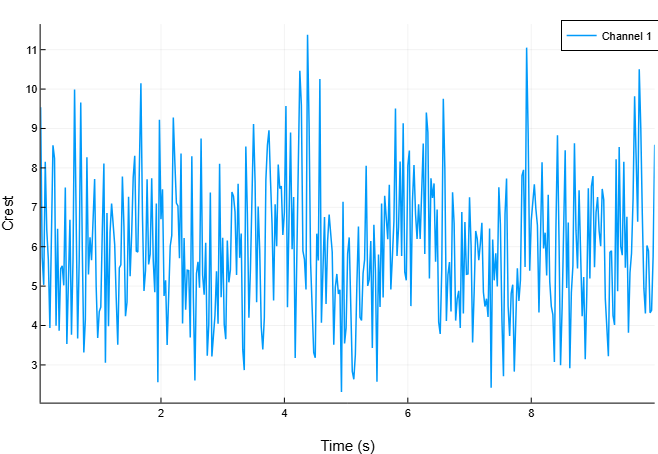
([9.538007545680625, 5.730876827698805, 5.032509222116753, 8.153962933846854, 6.409421405881727, 5.675496154818911, 3.936388047909756, 6.4173265830507695, 8.571412474805326, 8.245914575869225 … 9.01887114861341, 6.801343613682713, 4.948170085776451, 4.303209591503631, 6.032361588552264, 5.892015558392096, 4.323588797979937, 4.386216853001777, 5.755291814282484, 8.589943998230682], [1.072192257755449, 0.7611738870970485, 0.6151487100923281, 0.694504549763681, 0.41087548375427874, 0.35978967731876343, 0.38720592502049855, 0.3867047677182591, 0.846628743616088, 0.5501511870614189 … 0.9982941134388452, 0.6086401775262335, 0.16918248208293274, 0.2568272244259427, 0.4861993272274322, 0.563021155034732, 0.48023412546096145, 0.37966201056426135, 0.5141970164720814, 1.0541601271133798], [0.11241260322141401, 0.1328197952917255, 0.12223498913601331, 0.08517386642522173, 0.06410492581705285, 0.06339351970369599, 0.0983657912552872, 0.06025948075318637, 0.09877353891259522, 0.06671803133534474 … 0.11068947510047597, 0.08948822645892963, 0.03419091889530009, 0.0596827133247307, 0.08059850526037807, 0.09555663074120903, 0.11107303397708311, 0.08655796630402203, 0.08934334401533499, 0.12272025607274167], Plot{Plots.PlotlyJSBackend() n=1})Algorithms
The spectral crest is calculated as described in [1]:
where
-
— spectral value in bin ;
-
and — band boundaries in bins, which are used to calculate the spectral crest.