instfreq
Estimation of the instantaneous frequency.
| Library |
|
Syntax
Function call
-
ifq = instfreq(___,Name=Value)— sets additional parameters for any of the previous syntaxes using arguments of the "name-value" type. You can specify the algorithm used to estimate the instantaneous frequency, or the frequency limits used in the calculation.
-
instfreq(___)— displays the estimated instantaneous frequency without output arguments.
Arguments
Input arguments
# x — input signal
+
vector | the matrix
Details
An input signal specified as a vector or matrix. If x — vector, then instfreq processes it as a single channel. If x is a matrix, then the function calculates the instantaneous frequency independently for each column and returns the result in the corresponding column of the function ifq.
| Data types |
|
| Support for complex numbers |
Yes |
#
fs —
sampling
rate
positive scalar
Details
The sampling rate, set as a positive scalar. The sampling rate is the number of samples per unit of time. If the unit of time is seconds, then the sampling frequency is indicated in Hz.
| Data types |
|
# tfd — time-frequency distribution
+
the matrix
# fd,td — frequency and time values for the time-frequency distribution
+
vectors
Details
Frequency and time values for the time-frequency distribution, specified as vectors. These input arguments are supported only when a value is selected. "tfmoment" for the argument Method.
| Data types |
|
Name-value input arguments
Specify optional argument pairs as Name=Value, where Name — the name of the argument, and Value — the appropriate value. Name-value arguments should be placed after the other arguments, but the order of the pairs does not matter.
# FrequencyLimits — frequency range
+
[0 fs/2] (default for real signals) | [-fs/2 fs/2] (default for complex signals) | two-element vector
Details
The frequency range specified as a two-element vector in Hz. If FrequencyLimits omitted, this default argument is [0 fs/2] for real signals and [-fs/2 fs/2] for complex signals. This argument is supported only when a value is selected. "tfmoment" for the argument Method.
| Data types |
|
# Method — calculation method
+
"tfmoment" (by default) | "hilbert"
Details
The calculation method specified as "tfmoment" or "hilbert".
-
"tfmoment"— calculates the instantaneous frequency as the first conditional spectral moment of the time-frequency distributionx. IfxIt has uneven sampling, the function interpolates the signal onto a uniform grid to calculate instantaneous frequencies. -
"hilbert"— calculates the instantaneous frequency as a derivative of the phase of the analytical signalx, found using the Hilbert transform. This method accepts only uniformly sampled valid signals and does not support time-frequency distribution input data.
# out — type of output data
+
:data (by default) | :plot
Details
Type of output data:
-
:data— the function returns data; -
:plot— the function returns a graph.
Output arguments
# ifq — instantaneous frequency
+
vector | the matrix
Details
The instantaneous frequency returned as a vector or matrix with the same dimensions as the input data.
| Data types |
|
# t — frequency time estimates
+
the real vector
Details
Frequency time estimates returned as a real vector.
| Data types |
|
Examples
Instantaneous frequency of an unsteady signal
Details
We will generate a signal with a sampling frequency 5 kHz duration 4 seconds. The signal consists of a set of pulses of decreasing duration, separated by areas of amplitude and frequency fluctuations with a tendency to increase. Let’s plot the signal.
Pkg.add(["SpecialFunctions", "SignalAnalysis"])
using SpecialFunctions, SignalAnalysis
import EngeeDSP.Functions: instfreq

fs = 5000
t = 0:1/fs:4-1/fs

s = besselj.(0, 1000 .* (sin.(2*pi*t.^2/8).^4))

plot(t, s)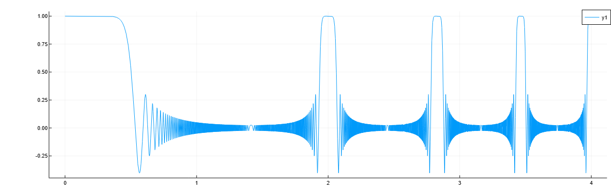
Let’s estimate the time-dependent frequency of the signal as the first moment of the power spectrogram. Let’s build a power spectrogram and superimpose an instantaneous frequency on it.
instfreq(s, fs, out=:plot)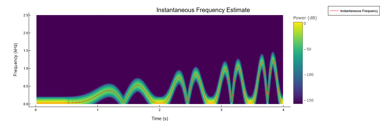
The instantaneous frequency of a complex-valued signal
Details
We will generate a complex-valued signal consisting of a chirp with a sinusoidally varying frequency. The signal is sampled at the frequency 3 kHz during 1 seconds, and white Gaussian noise is added to it.
import EngeeDSP.Functions: instfreq

fs = 3000
t = 0:1/fs:1-1/fs
x = exp.(2im*pi*100*cos.(2*pi*2*t)) + randn(size(t))/100
Let’s estimate the time-dependent frequency of the signal as the first moment of the power spectrogram. This is the only method that the function instfreq supports for complex-valued signals. Let’s build a power spectrogram and superimpose an instantaneous frequency on it.
instfreq(x, t, out=:plot)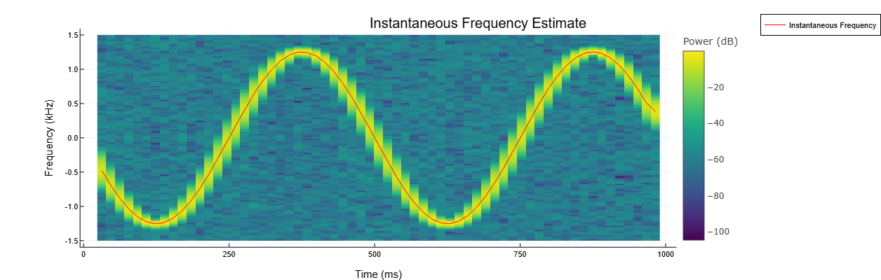
Instantaneous frequency of multi-channel signal
Details
Let’s create a two-channel signal sampled with a frequency 1 kHz during 2 seconds, consisting of two channels.
-
In the first channel, the instantaneous frequency changes over time in the form of a sawtooth wave, the maximum of which falls on
75% of the period. -
In the second channel, the instantaneous frequency changes over time in the form of a square wave with a fill factor
30.
import EngeeDSP.Functions: instfreq, sawtooth, square

fs = 1000
t = 0:1/fs:2
x = [sawtooth.(2*pi*t, 0.75) square.(2*pi*t, 30)]

plot(t, x)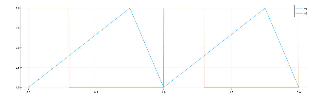
Calculate and display the instantaneous frequency.
instfreq(x, t, out=:plot)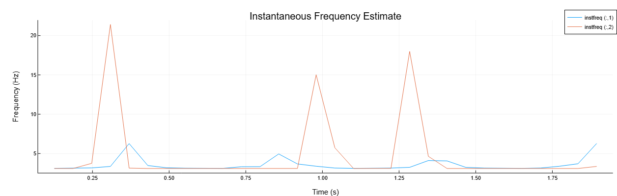
Instantaneous frequency of the chirp signal
Details
We will generate a chirp signal modulated by a Gaussian function. Setting the sampling frequency 2 kHz and signal duration 4 with.
import EngeeDSP.Functions: instfreq, pspectrum

fs = 2000
t = 0:1/fs:4-1/fs

q = real(chirp(0, 500, 4, fs)) .* exp.(-1.7*(t.-2).^2)

plot(t, q)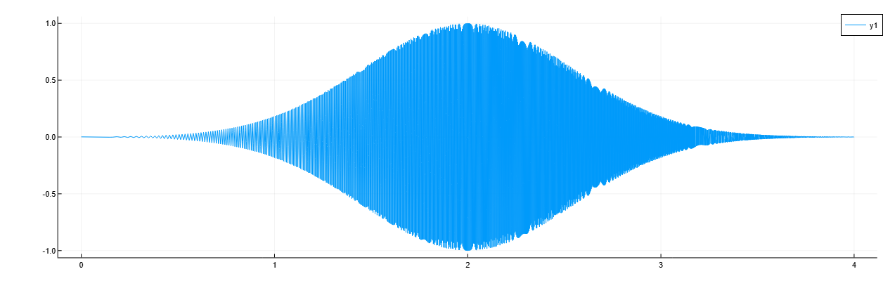
Using the function pspectrum with default settings for estimating the signal power spectrum. We use the estimate to calculate the instantaneous frequency.
p, f, t = pspectrum(q, fs, "spectrogram")

instfreq(p, f, t, out=:plot)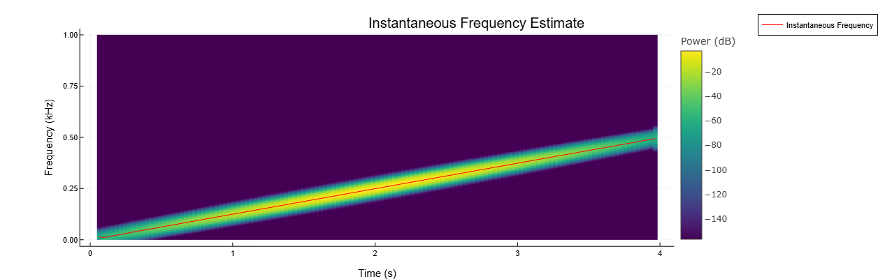
The instantaneous frequency of the sine wave
Details
We will generate a sinusoidal signal sampled with the frequency 1 kHz during 0.3 seconds and augmented with white Gaussian noise with variance 1/16. Let’s set the frequency of the sine wave 200 Hz. Estimate and display the instantaneous frequency of the signal.
import EngeeDSP.Functions: instfreq, pspectrum

fs = 1000
t = 0:1/fs:0.3-1/fs

x = sin.(2*pi*200*t) .+ randn(size(t))/4

instfreq(x, t, out=:plot)
Let’s estimate the instantaneous frequency of the signal again, but now we use the time-frequency distribution as input data.
p, fd, td = pspectrum(x, t, "spectrogram")

instfreq(p, fd, td, out=:plot)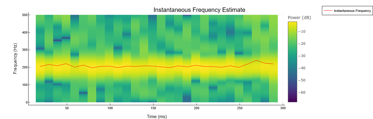
Additional Info
Instantaneous frequency
Details
The instantaneous frequency of an unsteady signal is a time—varying parameter that refers to the average of the frequencies present in the signal as it evolves [1], [2].
-
If for an argument
Methodvalue selected"tfmoment", then the functioninstfreqevaluates the instantaneous frequency as the first conditional spectral moment of the time-frequency distribution of the input signal. Function:-
Calculates the power spectrum of a spectrogram input signal using the function
pspectrumand uses the spectrum as a time-frequency distribution. -
Estimates the instantaneous frequency using the formula
-
-
If for an argument
Methodvalue selected"hilbert", then the functioninstfreqevaluates the instantaneous frequency as a derivative of the phase of the analytical input signal. Function:-
Calculates the analytical signal input signal using the function
hilbertand uses the spectrum as a time-frequency distribution. -
Estimates the instantaneous frequency using the formula
where — the phase of the analytical input signal.
-
Literature
-
Boashash, Boualem. «Estimating and Interpreting the Instantaneous Frequency of a Signal. I. Fundamentals.» Proceedings of the IEEE® 80, no. 4 (April 1992): 520–538. https://doi.org/10.1109/5.135376.
-
Boashash, Boualem. «Estimating and Interpreting The Instantaneous Frequency of a Signal. II. Algorithms and Applications.» Proceedings of the IEEE 80, no. 4 (May 1992): 540–568. https://doi.org/10.1109/5.135378.