dtw
The distance between the signals using dynamic time distortion.
| Library |
|
Syntax
Function call
-
dist, ix, iy = dtw(x, y)— stretches two vectorsxandyon a common set of time points in such a way thatdist, the sum of the Euclidean distances between the corresponding points, was the smallest. To stretch the input data, the functiondtwrepeats each elementxandythe required number of times. Ifxandy— matrices, thendiststretches them by repeating their columns. In this casexandythey must have the same number of rows. The function also returns a general set of time points.ixandiy, or a distortion path such that the distance betweenx(ix)andy(iy)it was the least. Vectorsixandiythey have the same length. Each of them contains a monotonically increasing sequence in which the indexes of the elements of the corresponding signalxorythey are repeated the required number of times. Whenxandyare matrices,ixandiysuch thatx(:,ix)andy(:,iy)minimally separated.
-
_ = dtw(_, out=:plot)— plots the original and aligned signals.
Arguments
Input arguments
# x — input signal
+
vector | the matrix
Details
An input signal specified as a real or complex vector or matrix.
| Data types |
|
| Support for complex numbers |
Yes |
# y — input signal
+
vector | the matrix
Details
An input signal specified as a real or complex vector or matrix.
| Data types |
|
| Support for complex numbers |
Yes |
# maxsamp — width of the setup window
+
Inf (by default) | a positive integer scalar
Details
The width of the setup window, set as a positive integer scalar.
| Data types |
|
# metric — distance metric
+
"euclidean" (by default) | "absolute" | "squared" | "symmkl"
Details
The distance metric set as one of the values: "euclidean", "absolute", "squared" or "symmkl". If and are -measured signals, then the metric sets — the distance between -m countdown and -m countdown . Learn more about see Dynamic time conversion.
-
"euclidean"— the root of the sum of the squares of the differences, also known as the Euclidean metric or : -
"absolute"— the sum of absolute differences, also known as the distance of city blocks, the Manhattan metric, the taxi metric, or : -
"squared"— the square of the Euclidean metric, consisting of the sum of the squares of the differences: -
"symmkl"— symmetric Kullback—Leibler metric. This metric is only true for real and positive numbers. and :
Output arguments
# dist — minimum distance between signals
+
positive real scalar
Details
The minimum distance between the signals, returned as a positive real scalar.
# ix is the distortion path of the first signal
+
index vector | the index matrix
Details
The distortion path of the first signal, returned as a vector or matrix of indexes.
# iy is the distortion path of the second signal
+
index vector | the index matrix
Details
The distortion path of the second signal, returned as a vector or matrix of indexes.
Examples
Dynamic time conversion of a sinusoid signal with a linearly varying frequency and sinusoids
Details
Let’s create two real signals: a sinusoid with a linearly varying frequency and a sinusoid. We use dynamic time transformation to align the signals so that the sum of the Euclidean distances between their points is the smallest. We will display the aligned signals and the distance.
import EngeeDSP.Functions: dtw

x = cos.(2 * pi * (3 * (1:1000) / 1000) .^ 2)
y = cos.(2 * pi * 9 * (1:399) / 400)

dtw(x,y, out=:plot)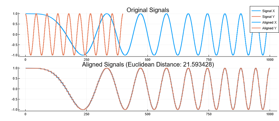
Change the frequency of the sine wave twice and repeat the calculations.
import EngeeDSP.Functions: dtw

x = cos.(2 * pi * (3 * (1:1000) / 1000) .^ 2)
y = cos.(2 * pi * 18 * (1:399) / 400)

dtw(x,y, out=:plot)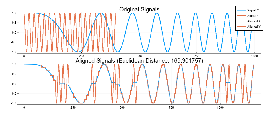
Additional Info
Dynamic time conversion
Details
Two signals with equivalent features arranged in the same order may look completely different due to the difference in the duration of their sections. Dynamic time transformation distorts these durations in such a way that the corresponding features appear in the same place on the common time axis, thereby emphasizing the similarity between the signals.
Consider two -three dimensional signals:
and
which contain and counts, respectively. The given distance between -the countdown and -the countdown , set in metric, dist stretches and for a common set of time points in such a way that the global measure of the distance between the signals is the smallest.
Initially, the function orders all possible values. into the grid of the form:

Then dist searches for a path through a lattice parameterized by two sequences of the same length, ix and iy, such that
minimal.
Acceptable paths dist they start in , end in and they represent combinations of moves of the "chess king":
-
vertical stroke: ;
-
horizontal stroke: ;
-
move diagonally: .
This structure ensures that any acceptable path aligns all signals, does not skip samples, and does not repeat signal features. In addition, the desired path runs close to the diagonal line drawn between and . This is an additional limitation imposed by the argument maxsamp, ensures that the distortion compares sections of the same length and does not overtake outliers.
Possible path through the grid:

The following paths are not allowed:
-
Does not align all signals:

-
Skips counts:

-
Turns back, repeating the element:

Literature
-
Paliwal, K. K., Anant Agarwal, and Sarvajit S. Sinha., A Modification over Sakoe and Chiba’s Dynamic Time Warping Algorithm for Isolated Word Recognition. Signal Processing. Vol. 4, 1982, pp. 329–333.
-
Sakoe, Hiroaki, and Seibi Chiba., Dynamic Programming Algorithm Optimization for Spoken Word Recognition. IEEE® Transactions on Acoustics, Speech, and Signal Processing. Vol. ASSP-26, No. 1, 1978, pp. 43–49.