falltime
The decay time of the negative edges of two-level signals.
| Library |
|
Syntax
Function call
-
_ = falltime(_, Name,Value)— returns the fall-off time with additional parameters specified by one or more arguments of the typeName,Value.
Arguments
Input arguments
# fs — sampling frequency, Hz
+
scalar
Details
The sampling frequency in Hz, set as a positive real scalar.
Name-value input arguments
Specify optional argument pairs in the format Name, Value, where Name — the name of the argument, and Value — the appropriate value. Name-value arguments should be placed after other arguments, but the order of the pairs does not matter.
Use commas to separate the name and value, and Name put it in quotation marks.
Example: f = falltime([4,3,2,1], "PercentReferenceLevels", [30 60]).
# PercentReferenceLevels — reference levels as a percentage of the signal amplitude
+
[10 90] (by default) | A two-element vector is a string
Details
Reference levels as a percentage of the signal amplitude, set as a two-element positive vector string. The elements of the row vector correspond to the low and high reference levels as a percentage. A high state level is defined as 100%, and low is like 0%. For more information, see [percentage-reference-levels].
# StateLevels — low and high state levels
+
A two-element vector is a string
Details
Low and high state levels, specified as a two-element vector string. The first and second elements of the vector correspond to low and high levels of states.
# Tolerance — upper and lower bounds of the state levels
+
2 (by default) | scalar
Details
The upper and lower bounds of the state levels, defined as a real positive scalar. For more information, see State level tolerances.
# out — type of output data
+
:data (by default) | :plot
Details
Type of output data:
-
:data— the function returns data; -
:plot— the function returns a graph.
Output arguments
# f — duration of the negative edge
+
vector
# lt — points of intersection of the lower reference level
+
vector
Details
The points of intersection of the lower reference level, returned as a vector. Vector lt It contains the time points when the negative edge crosses the lower reference level. By default, the lower value of the reference level is 10% from the reference level. You can change the default values of the reference levels by specifying the argument PercentReferenceLevels.
# ut — points of intersection of the upper reference level
+
vector
Details
The points of intersection of the upper reference level, returned as a vector. Vector ut It contains the time points when the negative edge crosses the upper reference level. By default, the upper value of the reference level is 90% from the reference level. You can change the default values of the reference levels by specifying the argument PercentReferenceLevels.
# ll — lower reference level
+
scalar
Details
The lower reference level in units of the signal amplitude, returned as a real numeric scalar.
By default, the lower value of the reference level is 10% from the reference level. You can change the default values of the reference levels by specifying the argument PercentReferenceLevels.
# ul — upper reference level
+
scalar
Details
The upper reference level in units of the signal amplitude, returned as a real numeric scalar.
By default, the upper value of the reference level is 90% from the reference level. You can change the default values of the reference levels by specifying the argument PercentReferenceLevels.
Examples
Signal decay time
Details
Calculate the signal decay time.
import EngeeDSP.Functions: falltime
f = falltime([4,3,2,1], "PercentReferenceLevels", [30 60], out=:data)
(0.5940000000000003, 3.391, 2.7969999999999997, 1.609, 2.2030000000000003)Let’s print a graph.
import EngeeDSP.Functions: falltime
f = falltime([4,3,2,1], "PercentReferenceLevels", [30 60], out=:plot)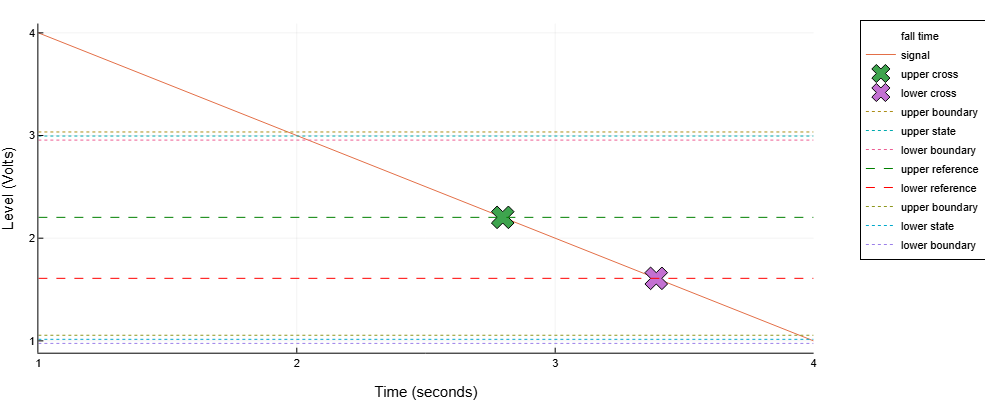
The decay time of a two-level signal
Details
Let’s determine the decay time of the two-level signal using the default values of the reference levels. 10% and 90%. Note the time of decline on the signal graph.
t = [0, 2.5000e-07, 5.0000e-07, 7.5000e-07, 1.0000e-06, 1.2500e-06, 1.5000e-06, 1.7500e-06, 2.0000e-06, 2.2500e-06, 2.5000e-06, 2.7500e-06, 3.0000e-06,
     3.2500e-06, 3.5000e-06, 3.7500e-06, 4.0000e-06, 4.2500e-06, 4.5000e-06, 4.7500e-06, 5.0000e-06, 5.2500e-06, 5.5000e-06, 5.7500e-06, 6.0000e-06,
     6.2500e-06, 6.5000e-06, 6.7500e-06, 7.0000e-06, 7.2500e-06, 7.5000e-06, 7.7500e-06, 8.0000e-06, 8.2500e-06, 8.5000e-06, 8.7500e-06, 9.0000e-06,
     9.2500e-06, 9.5000e-06, 9.7500e-06]

x = [2.3026, 2.2907, 2.2628, 2.3515, 2.2769, 2.2981, 2.3281, 2.3088, 2.2934, 2.2302, 2.2527, 2.3326, 2.2343, 2.2934, 2.3041, 2.2866, 2.3062,
     2.3055, 2.2707, 2.1992, 2.4520, -0.1271, 0.1181, -0.0250, -0.0227, -0.0061, -0.0216, -0.0125, 0.0085, -0.0031, 0.0175, -0.0202, 0.0273,
     0.0227, 0.0199, 0.0644, -0.0326, 0.0011, 0.0162, -0.0264]

import EngeeDSP.Functions: falltime

falltime(x, out=:plot)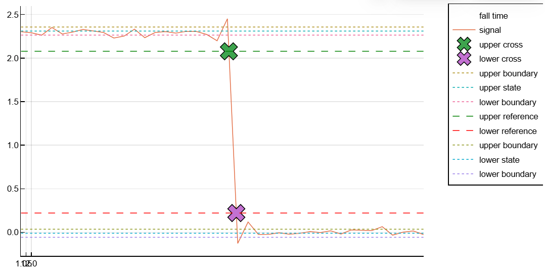
Again, we will determine the time of decline and indicate approximate time points. t. Let’s draw the result on a new graph.
falltime(x, t, out=:plot)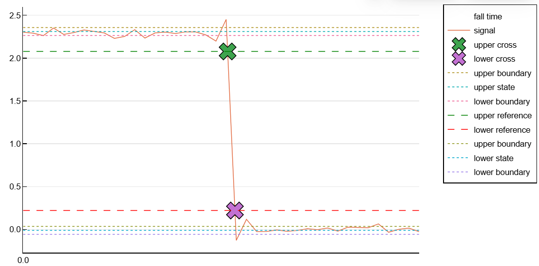
The time of decline at the reference levels of 20% and 80%
Details
Let’s calculate the decay time of a two-level signal using reference levels. 20% and 80%. Let’s plot the signal graph and indicate the time of decline on it.
falltime(x, "PercentReferenceLevels", [20 80], out=:plot)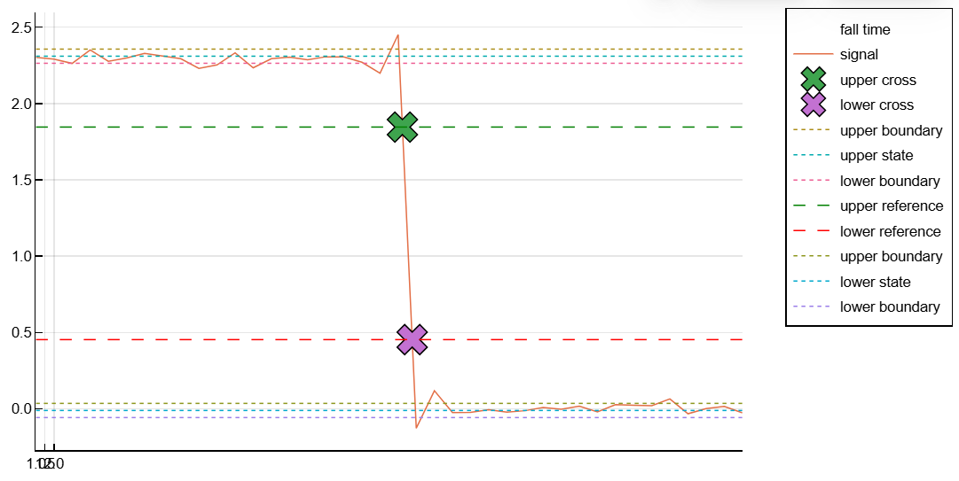
The time of decline, the time points of the reference level, and the reference levels
Details
For a two-level signal, we will determine the time of decline, the time points of the reference level and the reference levels. We will specify the time points of the sample t.
f, lt, ut, ll, ul = falltime(x, t, out=:plot)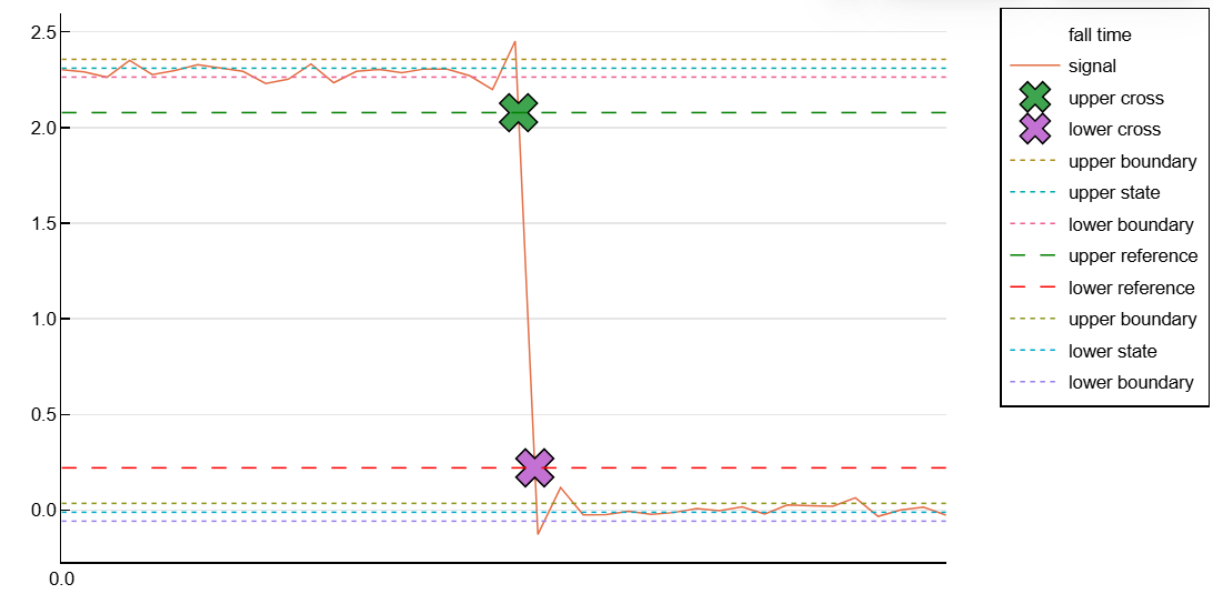
Let’s calculate the decline time as the difference between the moments of the lower and upper reference levels.
print("Fall time is ", lt-ut, " seconds")Fall time is 1.7999999999999828e-7 seconds
Additional Info
The front of the signal
Details
To determine the front, the function falltime evaluates the state levels of the input signal using the histogram method. The function defines all regions that intersect the lower boundary of the high state and the upper boundary of the low state. The boundaries of low and high states are expressed as the state level plus or minus a multiple of the difference between the state levels.
The negative front
Details
The negative edge in a two—level signal is the transition from a high-level state to a low-level state. If the signal is differentiable in the vicinity of the front, the equivalent definition is a front with a negative first derivative.
Percentage reference levels
Details
If — this is a low state, — high condition, eh — the upper percentage reference level, then the signal value corresponding to the upper percentage reference level is
If — this is the lower percentage reference level, then the signal value corresponding to the lower percentage reference level is
State level tolerances
Details
You can specify the lower and upper bounds of the states for each state level. Define boundaries as the state level plus or minus a scalar value that is a multiple of the difference between high and low states. To set a useful tolerance range, specify a scalar as a small number, for example 2/100 or 3/100. In the general case, the area for a low state, it is defined as
where — low condition, — high condition. Replace the first term in the equation with to get the tolerance area for a high condition.