powerbw
Power bandwidth.
| Library |
|
Syntax
Function call
-
bw = powerbw(___,freqlims,r)— defines the frequency range in which the reference level is calculated. This syntax can include any combination of input arguments from the previous options, provided that the second input argument is eitherFs, orf. If the second input argument is passed as empty,powerbwassumes a normalized frequency. The function calculates the frequency difference between the points where the spectrum falls below the reference level byrdB or reaches the end point.
-
powerbw(___)— without output arguments, plots the SPM or power spectrum in the current graph window and annotates the bandwidth.
Arguments
Input arguments
# x — input signal
+
vector | the matrix
Details
An input signal specified as a vector or matrix. If x — vector, it is considered as a single channel. If x — the matrix, then the function powerbw calculates the power bandwidth independently for each column. x it must be finite-valued.
| Data types |
|
#
Fs —
sampling
rate
positive real scalar
Details
The sampling frequency, set as a positive real scalar. The sampling rate is the number of samples per unit of time. If time is measured in seconds, then the sampling frequency is indicated in hertz.
| Data types |
|
# pxx — spectral power density
+
vector | the matrix
Details
An estimate of the spectral power density (SPM), defined as a vector or matrix. If pxx — one-sided evaluation, then it must correspond to the actual signal. If pxx — the matrix, then powerbw calculates the bandwidth of each column pxx regardless.
The power spectral density should be expressed in linear units, not in decibels. Use the function db2pow to convert decibel values to power values.
| Data types |
|
# f — frequencies
+
vector
Details
Frequencies specified as a vector. If the first element is f equal to 0 Then powerbw assumes that the spectrum is a one-way spectrum of a real signal. In other words, the function doubles the power value in the zero frequency bin, aiming for the point 3 dB.
| Data types |
|
# sxx — power spectrum estimation
+
vector | the matrix
Details
An estimate of the power spectrum, specified as a vector or matrix. If sxx — the matrix, then powerbw calculates the bandwidth of each column sxx regardless.
The power spectrum should be expressed in linear units, not in decibels. Use the function db2pow to convert decibel values to power values.
| Data types |
|
# rbw — resolution band
+
positive scalar
Details
The resolution band, set as a positive scalar. The resolution band is the product of two quantities: the frequency resolution of the discrete Fourier transform and the equivalent noise band of the window used to calculate the SPM.
| Data types |
|
# freqlims — frequency limits
+
two-element vector
Details
Frequency limits set as a two-element vector of real values. If the argument is freqlims If set, the reference level will be the average power level in the reference band. If the argument is freqlims If not specified, the reference level will be the maximum power level in the spectrum. Meaning freqlims must be within the target band.
| Data types |
|
# r — power level drop
+
10*log10(2) (by default) | positive real scalar
Details
The power level drop, given as a positive real scalar, expressed in dB.
| Data types |
|
Name-value input arguments
# out — type of output data
+
:data (default) | :plot
Details
Type of output data:
-
:data— the function returns data; -
:plot— the function returns a graph.
Examples
Bandwidth-limited signals
Details
We will generate a signal whose SPM resembles the frequency response of a bandpass FIR filter. 88-th order with normalized cutoff frequencies rad/countdown and rad/countdown.
import EngeeDSP.Functions: fir1

d = fir1(88, [0.25 0.45])
Calculate the occupied signal band at the level of 3 dB. We will specify the average power in the range from as a reference level. rad/countdown to rad/countdown. Let’s build a schedule for the SPM.
import EngeeDSP.Functions: powerbw

powerbw(d, [], [0.2 0.6]*pi, 3, out=:plot)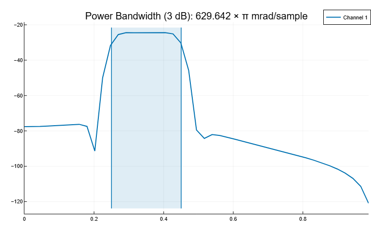
We will output the bandwidth, its lower and upper limits, as well as the bandwidth power. Specifying the sampling rate it is equivalent to leaving it unidentified.
bw, flo, fhi, power = powerbw(d, 2π, [0.2, 0.6] * π)
println([" bw"; "flo"; "fhi"] .* " = " .* string.([bw; flo; fhi] / π) .* "π")
[" bw = 0.20047359178514887π", "flo = 0.24995529776303813π", "fhi = 0.450428889548187π"]import EngeeDSP.Functions: bandpower
println("power = ", round((power/bandpower(d)*100)[1], digits=1), "% of total")power = 96.9% of totalAdd a second channel with normalized cutoff frequencies rad/countdown and rad/count and an amplitude of one tenth of the amplitude of the first channel.
d = [d fir1(88, [0.5 0.8])/10]Let’s calculate the bandwidth of a two-channel signal at the level of 6 dB. We will specify the maximum power level of the spectrum as a reference level.
powerbw(d, [], [], 6, out=:plot)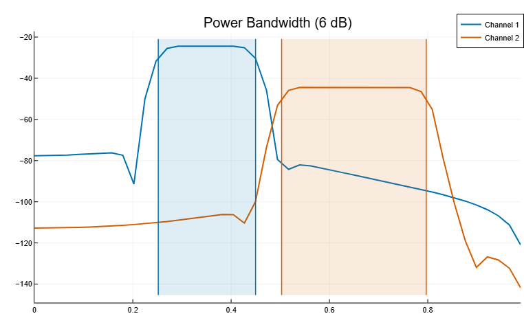
Let’s output the bandwidth of each channel at the level of 6 dB, as well as the lower and upper limits.
bw, flo, fhi = powerbw(d, [], [], 6)
bds = [bw[1] bw[2]; flo[1] flo[2]; fhi[1] fhi[2]]
labels = [" bw", "flo", "fhi"]

for channel in 1:2
    for i in 1:3
        println(labels[i] * " (ch_$channel) = $(round(bds[i, channel] / π, digits=5))π")
    end
end
bw (ch_1) = 0.19794π
flo (ch_1) = 0.25176π
fhi (ch_1) = 0.44971π
bw (ch_2) = 0.29418π
flo (ch_2) = 0.50271π
fhi (ch_2) = 0.79689πThe bandwidth of chirp signals at the 3 dB level
Details
Generate 1024 sampling of a chirp signal with a frequency 1024 kHz. The initial frequency of the chirp signal is 50 kHz, and at the end of the sample it reaches 100 kHz. Add white Gaussian noise so that the signal-to-noise ratio is 40 dB.
import EngeeDSP.Functions: chirp, std, powerbw

nSamp = 1024
Fs = 1024e3
SNR = 40

t = (0:nSamp-1)'/Fs

x = chirp(t, 50e3, nSamp/Fs, 100e3)
x = x .+ randn(size(x)) * std(x).S / (10^(SNR/20));
Let’s estimate the signal bandwidth at 3 dB and mark it on the spectrum graph.
powerbw(x, Fs, out=:plot)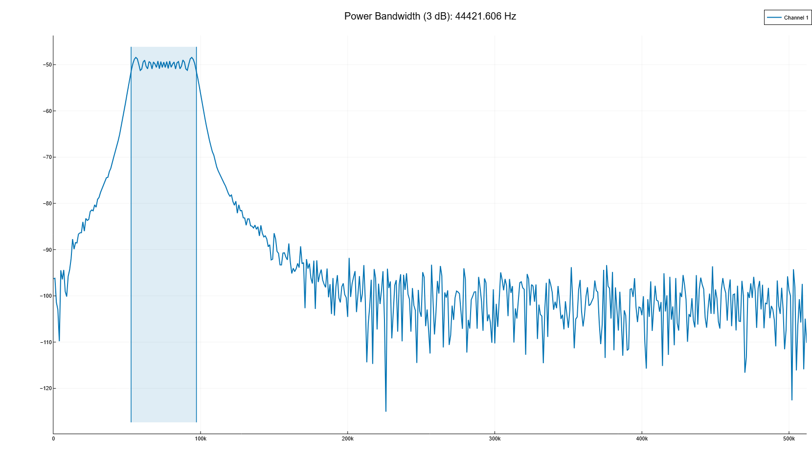
Let’s generate another chirp signal. Setting the initial frequency 200 kHz, the final frequency 300 kHz and an amplitude that is twice the amplitude of the first signal. Add white Gaussian noise.
x2 = 2 * chirp(t, 200e3, nSamp/Fs, 300e3)
x2 = x2 .+ randn(size(x2)) * std(x2).S / (10^(SNR/20));
Let’s combine the chirp signals to get a two-channel signal. Let’s estimate the bandwidth of each channel at 3 dB.
y = powerbw([x; x2]', Fs)([44397.27005796786, 92225.32672086824], [52812.86939829475, 203906.69033994916], [97210.13945626261, 296132.0170608174], [0.4626064585350288, 1.8949783295500369])Note the bandwidth of the two channels at the 3 dB on the spectrum graph.
powerbw([x; x2]', Fs, out=:plot);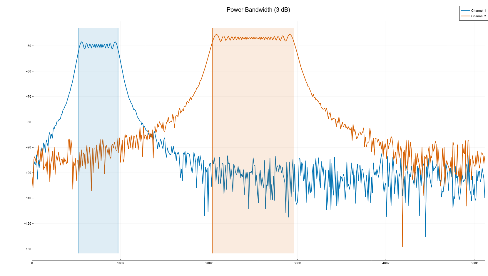
Add up the two channels to form a new signal. Let’s estimate the power spectrum and mark the bandwidth at 3 dB.
powerbw(x+x2, Fs, out=:plot)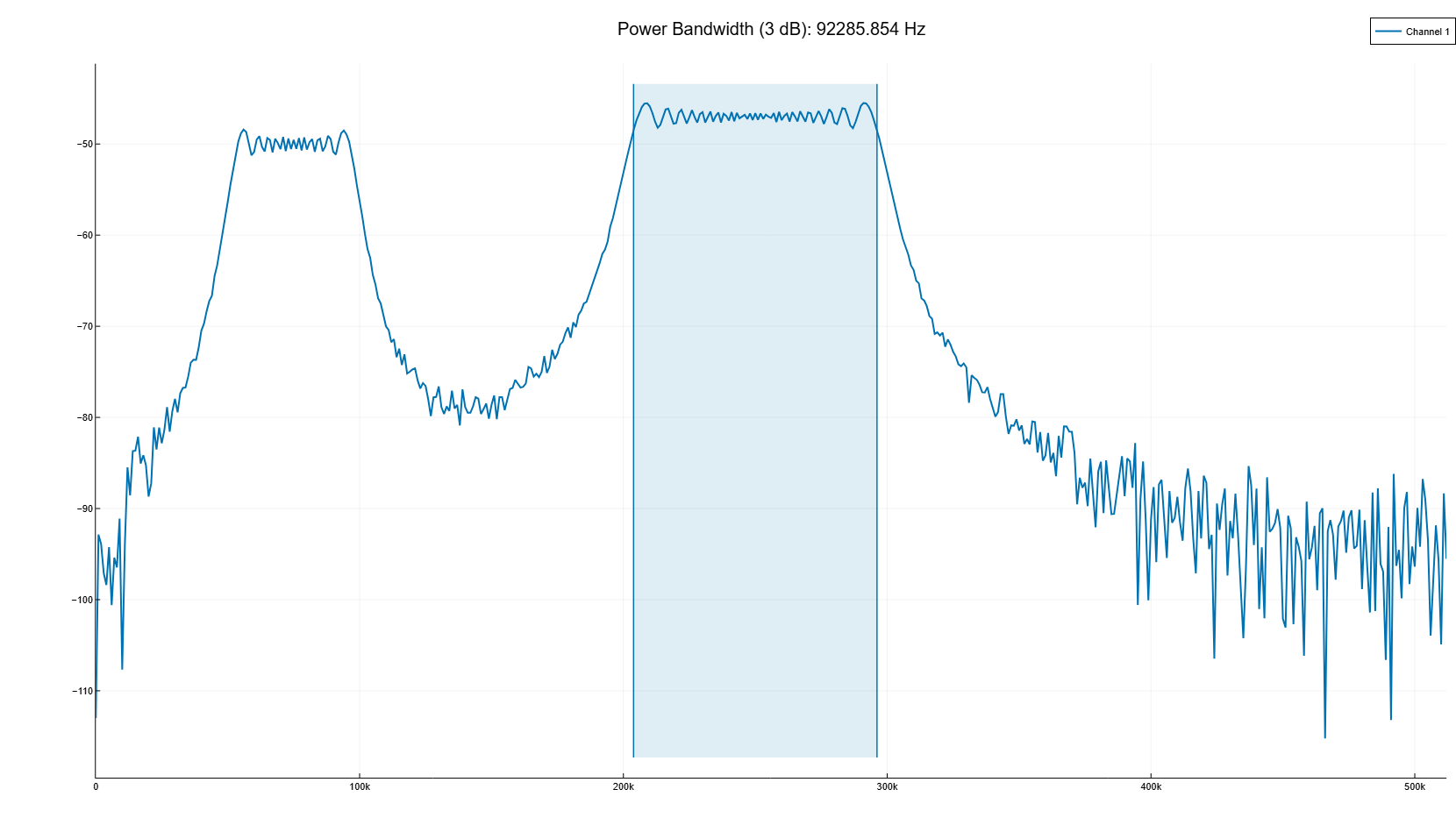
The bandwidth of sinusoidal signals at the 3 dB level
Details
Generate 1024 counting the sinusoid by frequency 100.123 kHz, sampled at the frequency 1024 kHz. Add white Gaussian noise so that the signal-to-noise ratio is 40 dB. To get reproducible results, restart the random number generator.
import EngeeDSP.Functions: pspectrum
using Random

nSamp = 1024
Fs = 1024e3
SNR = 40
Random.seed!("default")

t = (0:nSamp-1)'/Fs

x = sin.(2*pi*t*100.123e3)
x = x .+ randn(size(x)) * std(x).S / (10^(SNR/20));
Using the function pspectrum to calculate the signal power spectrum. Let’s estimate the signal bandwidth at 3 dB and mark it on the graph of the spectrum.
p, f, t1 = pspectrum(x, Fs)

powerbw(p, f, out=:plot);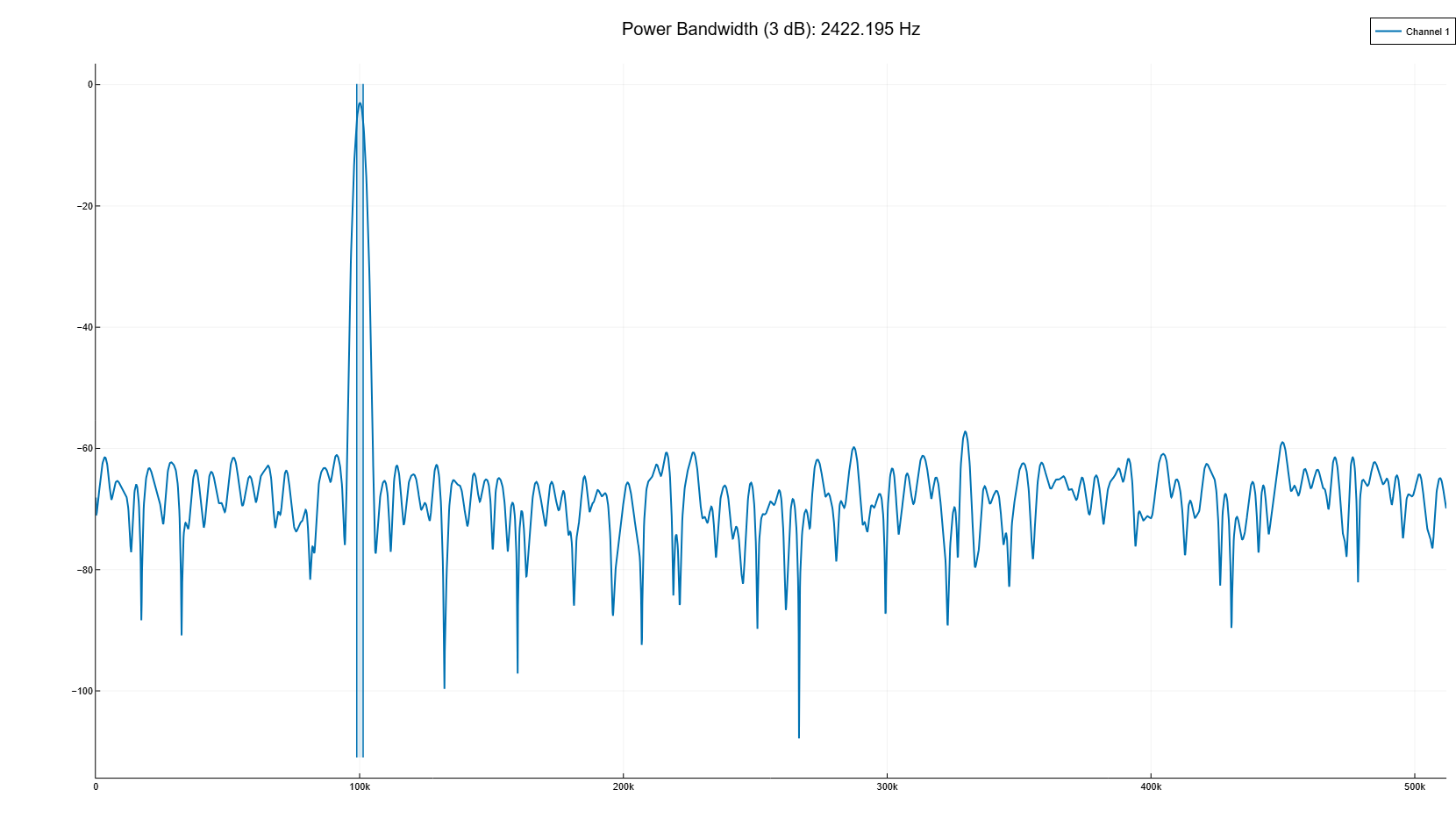
Let’s generate another sinusoid, this time with a frequency of 257.321 kHz and an amplitude twice the amplitude of the first sine wave. Add white Gaussian noise.
x2 = 2 * sin.(2*pi*t*257.321e3)
x2 = x2 .+ randn(size(x2)) * std(x2).S / (10^(SNR/20));
Combine the sinusoids to get a two-channel signal. Let’s estimate the power spectrum of each channel and use the result to determine the bandwidth at the level of 3 dB.
p, f, t = pspectrum([x; x2]', Fs)

y = powerbw(p, f)
([2422.1946183990804, 2421.005680883798], [98912.42452799428, 256110.8536321677], [101334.61914639336, 258531.8593130515], [981.6720278356812, 3921.693919771026])Note the bandwidth of the two channels at the 3 dB on the spectrum graph.
powerbw(p, f, out=:plot);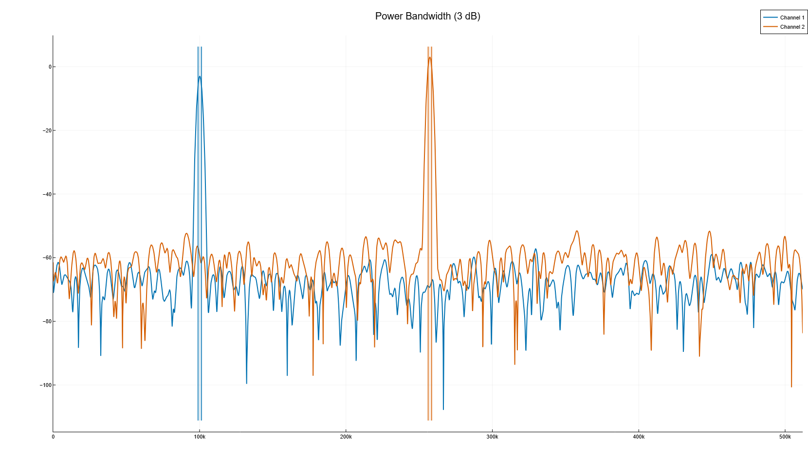
Add up the two channels to form a new signal. Let’s estimate the power spectrum and mark the bandwidth at 3 dB.
p, f, t = pspectrum(x+x2, Fs)

powerbw(p, f, out=:plot);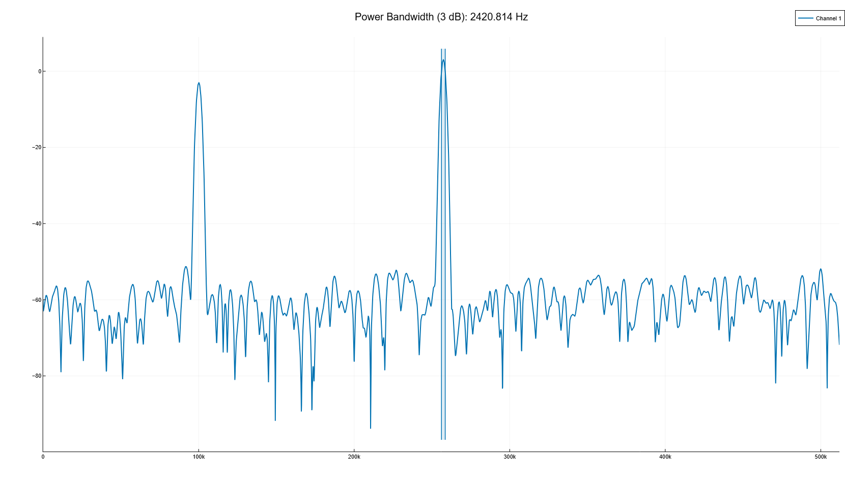
Algorithms
To determine the bandwidth at the level of 3 dB function powerbw Calculates an estimate of the periodogram’s power spectrum using a rectangular window and uses the highest estimate as a reference level. Bandwidth is the frequency difference between points where the spectrum drops by at least 3 dB relative to the reference level. If the signal reaches one of its endpoints before descending to 3 dB, function powerbw uses this endpoint to calculate the difference.
The same bandwidth value per level 3 dB, bw, can be obtained from the signal x with sampling rate Fs in three ways.
Straight from the signal |
|
From the periodogram of the signal |
|
From the estimation of the spectral power (SPM Welch) of the signal |
|
Because powerbw It uses an intermediate representation to convert the input signal from the time domain to the frequency domain. The bandwidth of the returned power may vary depending on the signal conversion method, the number of DFT points, and the window size.
|