spectrogram

A spectrogram using the windowed Fourier transform.

Library

EngeeDSP

Syntax

Function call

s, f, time, p = spectrogram(x) — returns the Windowed Fourier Transform (OPF) of the input signal x. Each column s contains an estimate of short-term, time-localized frequency content x. Value s² It is a time-frequency representation spectrogram. x [1].

s, f, time, p = spectrogram(x, window) — additionally uses the argument window to split the signal into segments and perform window processing.

s, f, time, p = spectrogram(x, window,noverlap) — additionally uses the argument noverlap to overlap adjacent segments.

s, f, time, p = spectrogram(x, window, noverlap, nfft) — additionally uses the argument nfft to set the number of points in the discrete Fourier transform.

s, f, time, p = spectrogram(x, window, noverlap, freq) — additionally uses the argument freq to set normalized or cyclic frequencies.

s, f, time, p = spectrogram(_, Name=Value) — uses arguments Name=Value in addition to any input arguments provided in the previous syntaxes.

Arguments

Input arguments

# x — input signal

+ vector

Details

The input signal is set as a row vector or column vector.

Типы данных	`Float32`, `Float64`
Support for complex numbers	Yes

# window — window

+ a positive integer | vector

Details

The window value specified as a positive integer, row vector, or column vector. Use window to split the signal into segments:

If window — an integer, then spectrogram divides x into segments of length window and uses a Hamming window of the same length for each segment.
If window — vector, then spectrogram divides x into segments of the same length as the vector, and uses a window for each segment. window.

If the length is x if it cannot be precisely divided into an integer number of segments without overlapping samples, then x it is truncated accordingly.

If you do not specify window Then spectrogram uses the Hamming window in such a way that x It is divided into eight segments with no overlapping counts.

# noverlap — number of intersecting points

+ a non-negative integer

Details

The number of intersecting signal points, set as a non-negative integer.

If the argument is window — scalar, the value of the argument noverlap must be less than the value of the argument window.
If the argument is window — vector, the value of the argument noverlap must be less than the value of the argument length. window.

If you do not specify the value of the argument noverlap, the spectrogram uses a number that gives 50% overlaps between segments. If the segment length is not specified, the function sets the value noverlap an equal , where — the length of the input signal, and the symbols denote rounding down.

# nfft is the number of points in the discrete Fourier transform
a positive integer

Details

The number of points in the discrete Fourier transform, given as a positive integer scalar.

If you do not specify a value for nfft, then the spectrogram will use the value , where , symbols denote rounding up, while:

window if the argument is window — scalar;
length(window) if the argument is window — vector.

# freq — normalized/cyclic frequencies

+ the real vector

Details

Frequency values specified as a real vector. The type of set frequencies depends on the value of the argument fs:

If the value of the input argument is fs If not specified, the default frequencies are considered normalized.;
If the value of the input argument is fs If indicated, the frequencies are considered cyclic.

You can set either freq as a vector, either nfft as a positive integer. Using these arguments at the same time will give an error.

Name-value input arguments

Specify optional argument pairs in the format Name=Value, where Name — the name of the argument, and Value — the appropriate value. Type arguments Name=Value they should be placed after the other arguments, but the order of the pairs does not matter.

# fs — sampling rate
1 Hz (by default) | a positive real number

Details

The sampling rate, set as a positive scalar. The sampling rate is the number of samples per unit of time. If the unit of time is seconds, then the sampling frequency is expressed in Hz.

# freqrange — frequency range of energy spectrum density estimation

+ "onesided" | "twosided"

Details

The frequency range for estimating the energy spectrum density (PSD), given as "onesided" or "twosided".

For signals with real values, the default value is "onesided". For complex signals, the default value is "twosided", and specifying the value "onesided" leads to an error.

Meaning "onesided" — returns a one-way spectrogram of the real input signal.
- If the value of the argument is nfft even, then the argument p has nfft/2 + 1 rows and is calculated on the interval [0, π] radians to count.
- If the value of the argument is nfft If it’s an odd number, then p has (nfft + 1)/2 lines and spacing [0, π) radians to count. If you specify fs, then the intervals will be respectively [0, fs/2] cycles per unit of time and [0, fs/2) cycles per unit of time.
Meaning "twosided" — returns a two-way spectrogram of a real or complex signal. Argument p has nfft rows and is calculated on the interval [0, 2π) radians to count. If you specify an argument fs, then the interval will have [0, fs) cycles per unit of time.

# centered — is the frequency range centered

+ false (by default) | true

Details

Enabling the centering of the frequency range, set as false or true.

# spectrumtype — scaling the energy spectrum density

+ "psd" (default) | "power"

Details

Scaling of the energy spectrum density (PSD), defined as "psd" or "power".

If the spectrum type is not specified or the value is specified "psd", then the function returns the spectral power density.

Meaning "power" scales each estimate of the energy spectrum density by the equivalent window noise band. The result is an estimate of the power at each frequency.

# freqloc — frequency display axis

+ "xaxis" (by default) | "yaxis"

Details

The frequency display axis, set as "xaxis" or "yaxis".

Meaning "xaxis" — frequency display along the axis and time on the axis .
Meaning "yaxis" — frequency display along the axis and time on the axis .

# MinThreshold — threshold of minimum values

+ −Inf (by default) | the real scalar

Details

The threshold value set as a real scalar in dB. The spectrogram zeroes out those elements s, for which 10 log₁₀(s) ≤ MinThreshold.

# OutputTimeDimension — time direction

+ "acrosscolumns" (by default) | "downrows"

Details

The time direction of the output data, set as "acrosscolumns" or "downrows". Set this argument to "downrows" if you want the time direction for the output arguments to be displayed in rows, and the frequency direction in columns. Set the value "acrosscolumns" if you want the time direction for the output arguments to be displayed in columns, and the frequency direction in rows.

# out — type of output data

+ :plot (by default) | :data

Details

Type of output data:

:data — the function returns data s, f, time and p;
:plot — the function builds a spectrogram.

If out = :plot, then you can additionally pass parameters to display the total heatmap(). For example, if you call spectrogram(x, c = cgrad([:black, :white], [0.1, 0.3, 0.8])), then the spectrogram will have gray colors instead of the standard ones.

Output arguments

# s is the discrete Fourier transform
the matrix

Details

A discrete Fourier transform returned as a matrix. The time increases across the columns of the matrix s, and the frequency increases line by line, starting from zero.

If x — signal length , then the matrix s has columns where
- noverlap window noverlap if window — scalar;
- noverlap length(window) noverlap if window — vector.
If x — material, eh nfft — even, then the matrix s has (nfft/2 + 1) lines.
If x — material, eh nfft — odd, then the matrix s has (nfft + 1)/2 lines.
If x — complex, then the matrix s has nfft lines.

If the parameter freqrange it matters "onesided", then the spectrogram outputs the values s It is in the positive Nyquist range and does not retain full power.

# f — cyclic frequencies

+ vector

Details

Cyclic frequencies returned as a vector. Vector length f is equal to the number of rows of the matrix s.

# time — points in time

+ vector

Details

The time points returned as a vector. Time values in t they correspond to the middle of each segment.

# p is the energy spectrum density

+ the matrix

Details

The energy spectrum density (PSD) or the power spectrum returned as a matrix.

If x — a real number, and freqrange omitted or set to value "onesided" Then p It contains a one-sided modified PSD periodogram or the power spectrum of each segment. The function multiplies the power by 2 on all frequencies except 0 and Nyquist frequencies to preserve the overall power.
If x is a complex number or if freqrange set to the value "twosided" or "centered" Then p It contains a two-sided modified PSD periodogram or the power spectrum of each segment.
If you specify a vector of normalized or cyclic frequencies in freq Then p It will contain a modified PSD periodogram or the power spectrum of each segment calculated at the input frequencies.

Examples

Default values for the spectrogram

Details

Generate samples of a signal representing the sum of sinusoids. The normalized frequencies of the sinusoids are rad/countdown and rad/countdown. A sinusoid with a higher frequency has in times the amplitude of the other sine wave.

import EngeeDSP.Functions: spectrogram
N = 1024
n = 0:N-1
w0 = 2pi / 5
x = sin.(w0 * n) .+ 10 * sin.(2 * w0 * n)

Let’s calculate the windowed Fourier transform using the default function parameters. Let’s build a spectrogram.

spectrogram(x,freqloc="yaxis")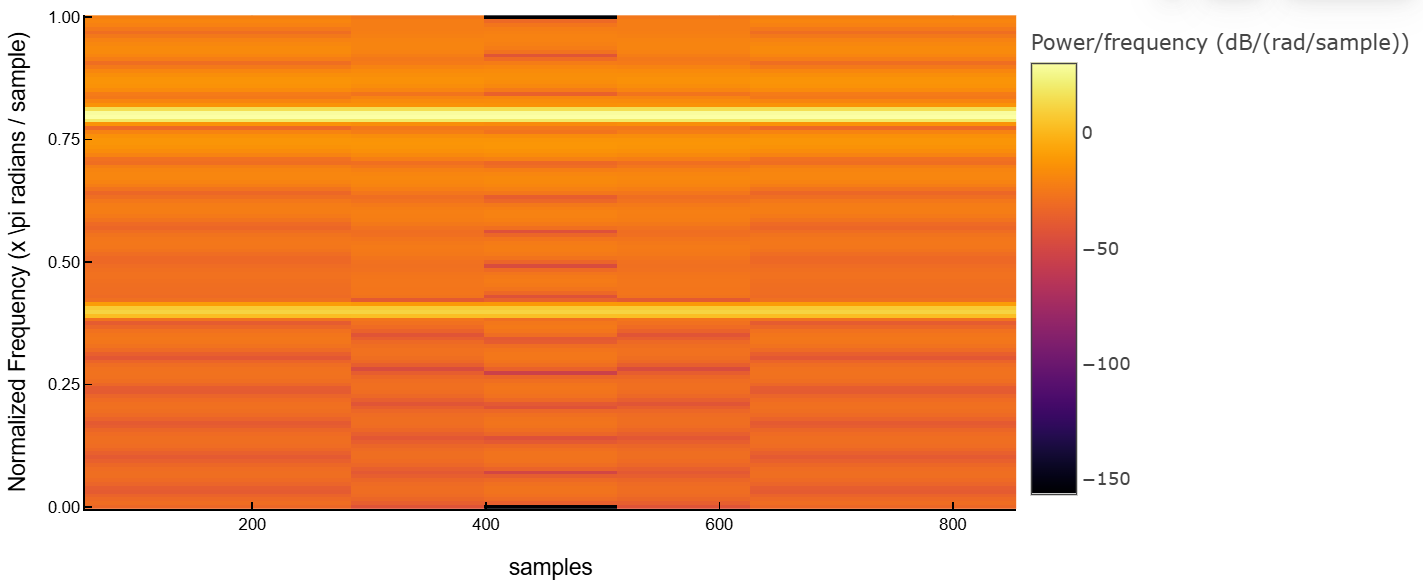

spectrogram 1

Complex signal spectrogram

Details

Generate 512 frequency modulation samples with sinusoidally varying frequency composition. Let’s calculate the centered two-way windowed Fourier transform of frequency modulation. Let’s divide the signal into segments by 32 reference points with overlap in 16 counts. Specify 64 discrete Fourier transform points. Let’s build a spectrogram.

import EngeeDSP.Functions: spectrogram
N = 512
n = collect(0:N-1)

x = @. exp(im*pi*sin(8*n/N)*32)
spectrogram(x, 32, 16, 64, centered = true, freqloc="yaxis")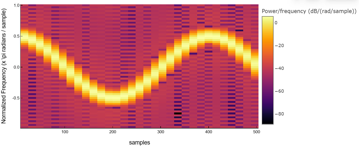

spectrogram 2

Let’s display the results as data.

spectrogram(x, 32, 16, 64, centered = true, freqloc="yaxis", out=:data)

(ComplexF64[-0.004799003568266007 - 0.0505661817205643im 0.04928181142575791 - 0.08168061694423136im … 0.06661413792128079 + 0.005582741943515573im 0.06563897996263357 - 0.03809302080510557im; 0.08251130568172917 - 0.009465091175966937im 0.01113491156754788 + 0.0019301579098507408im … -0.0033130937073331257 + 0.04853476281962177im 0.013263617768417113 + 0.025903864451430003im; … ; -0.009649405525420679 - 0.05239849276178002im 0.04401940995315085 - 0.0914065432314291im … 0.06820937107281076 - 6.325260894440854e-5im 0.06223032913485138 - 0.04414639111404428im; 0.08717673328273712 - 0.01888297777102288im 0.0132333274580263 + 0.0005901735083794213im … 0.002529248964486752 + 0.05007735729089752im 0.017119544189724056 + 0.024263377986849743im], [-3.043417883165112, -2.945243112740431, -2.84706834231575, -2.748893571891069, -2.650718801466388, -2.5525440310417067, -2.4543692606170255, -2.356194490192345, -2.2580197197676637, -2.1598449493429825  …  2.2580197197676637, 2.3561944901923453, 2.454369260617026, 2.5525440310417067, 2.6507188014663883, 2.748893571891069, 2.8470683423157497, 2.9452431127404313, 3.043417883165112, 3.1415926535897936], [2.5464790894703255 5.092958178940651 … 76.39437268410977 78.94085177358009], [3.3313443855835635e-5 0.00011750773553006685 … 5.770022477295285e-5 7.436932913915006e-5; 8.906550573571001e-5 1.6490579693362508e-6 … 3.0558345518866313e-5 1.0935898096347522e-5; … ; 3.665443356386854e-5 0.00013290498623780864 … 6.0074958410346855e-5 7.516942675213517e-5; 0.00010273510683279117 2.2657190730313684e-6 … 3.246341980220297e-5 1.1385977847041683e-5])

Additional Info

Windowed Fourier Transform (OPF)

Details

The windowed Fourier transform (OPF) is used to analyze changes in the frequency content of an unsteady signal over time. The value of the square of the OPF is known as the spectrogram of the time-frequency representation of the signal.

The OPF of the signal is calculated by sliding the analysis window lengths based on the signal and the calculation of the discrete Fourier transform (DFT) of each segment of the window data. The window slides over the original signal with an interval of counts, which is equivalent to counts of overlap between adjacent segments. Most window functions taper at the edges to avoid spectral ringing. The DFT of each segment with a window is added to a complex matrix containing the magnitude and phase for each point in time and frequency. The OPF matrix has columns where — signal length , and the symbols denote the rounding down function. The number of rows in the matrix is , the number of DFT points, for centered and two-sided transformations, and an odd number close to , for one-way transformations of real signals.

-th column of the OPF matrix contains a time-centered window data DFT :

spectrogram 1 en

If there are zeros in the windowed Fourier transform, its conversion to decibels leads to negative infinite values that cannot be plotted. To avoid this potential difficulty, the function spectrogram adds eps to the windowed Fourier transform when you call it without output arguments.

Literature

Boashash, Boualem, ed. «Time Frequency Signal Analysis and Processing: A Comprehensive Reference.» Second edition. EURASIP and Academic Press Series in Signal and Image Processing. Amsterdam and Boston: Academic Press, 2016.
Chassande-Motin, Éric, François Auger, and Patrick Flandrin. «Reassignment.» In Time-Frequency Analysis: Concepts and Methods. Edited by Franz Hlawatsch and François Auger. London: ISTE/John Wiley and Sons, 2008.
Fulop, Sean A., and Kelly Fitz. «Algorithms for computing the time-corrected instantaneous frequency (reassigned) spectrogram, with applications.» Journal of the Acoustical Society of America. Vol. 119, January 2006, pp. 360–371.
Oppenheim, Alan V., and Ronald W. Schafer, with John R. Buck. «Discrete-Time Signal Processing.» Second edition. Upper Saddle River, NJ: Prentice Hall, 1999.
Rabiner, Lawrence R., and Ronald W. Schafer. «Digital Processing of Speech Signals.» Englewood Cliffs, NJ: Prentice-Hall, 1978.