arburg
The parameters of the autoregression model with all poles are the Burg method.
| Library |
|
Arguments
Examples
Estimation of parameters using the Burg method
Details
We use the vector of coefficients of the generating polynomial to generate the process by filtering 1024 white noise samples. Reset the random number generator to get reproducible results. We use the Burg method to estimate the coefficients.
import EngeeDSP.Functions: randn,filter,arburg

A = [1 -2.7607 3.8106 -2.6535 0.9238]
y = filter(1,A,0.2*randn(1024,1))
arcoeffs = arburg(y,4)[1]
1×5 Matrix{Float64}:
1.0 -2.7743 3.84077 -2.68434 0.936008Generate 50 implementations of the process, changing the variance of the input noise each time. Let’s compare the variance calculated by the Burg method with the actual values.
nrealiz = 50
order = 4
noisestdz = rand(1, nrealiz) .+ 0.5
randnoise = randn(1024, nrealiz)
noisevar = zeros(1, nrealiz)

for k in 1:nrealiz
    y = filter(ones(1), A, noisestdz[k] * randnoise[:, k])
        arcoeffs,noisevar[k],e = arburg(y, order)

end

p=scatter(vec(noisestdz.^2), vec(noisevar),
        marker=:x,
        markerstrokecolor=:blue,
        xlabel="Input",
        ylabel="Estimated",
        title="Noise Variance",
        label="Single channel loop",
        legend=false)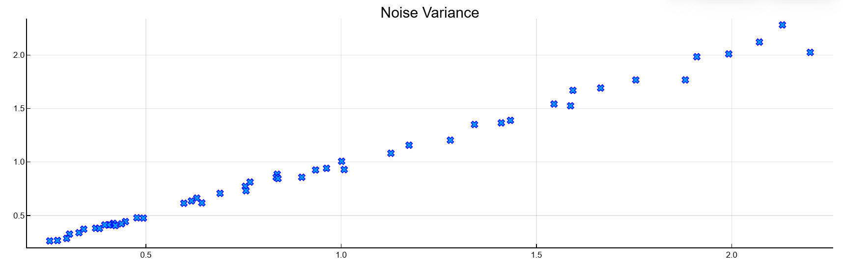
Let’s repeat the procedure using the multi-channel syntax of the function.
Y = filter(1,A,noisestdz.*randnoise)

coeffs,variances,e = arburg(Y,4)

scatter!(p,noisestdz.^2, variances,
        marker=:circle,
        markercolor=:transparent,
        markerstrokecolor=:green,
        markersize=10)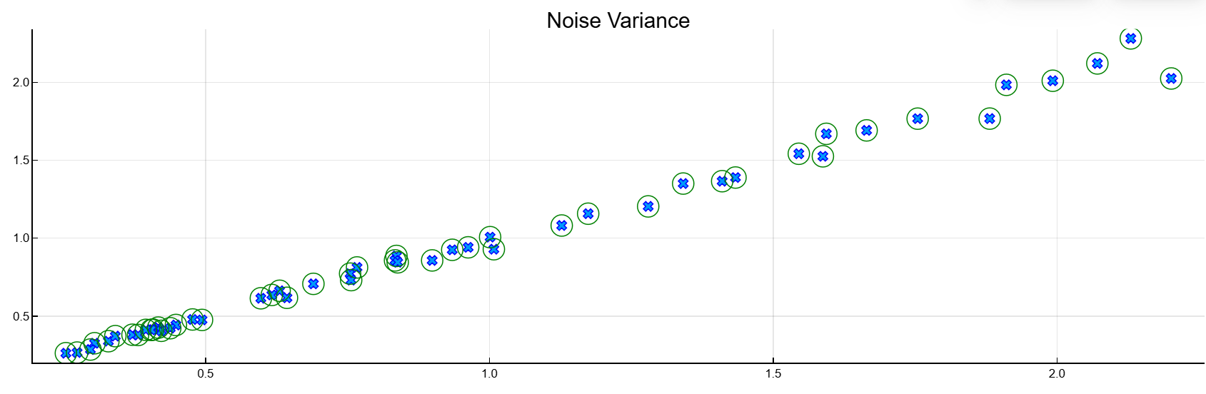
Additional Info
An autoregression model of the order of p
Details
In the autoregression model of the order ( ) the current output is a linear combination of the previous ones outputs plus a white noise input signal.
Weights on previous ones The outputs minimize the average quadratic error of the autoregression prediction. If — this is the current output value, and — this is an input signal with zero average white noise, then the model it has the form:
Algorithms
The Burg method calculates reflection coefficients and uses them for recursive estimation of autoregression parameters. The relations of recursion and the lattice filter describing the updating of forward and reverse prediction errors can be found in [1].