rlevinson
The Levinson—Durbin inverse recursion.
| Library |
|
Syntax
Function call
-
r,u,k,eEvolution = rlevinson(a,eFinal)— returns the autocorrelation sequencerfor a predictive filter with coefficients specified in the argumenta, and the power of the final prediction erroreFinal. It also returns a polynomial matrixurecursive predictive filter, reflection coefficientskand prediction errorseFinalfrom each iteration of the Levinson—Durbin inverse recursion.
Arguments
Input arguments
# a — coefficients of the predictive filter
+
vector
Details
Coefficients of the predictive filter, set as a vector.
|
The filter associated with If |
| Data types |
|
| Support for complex numbers |
Yes |
# eFinal — the power of the final prediction error
+
scalar
Details
The power of the final prediction error, given as a scalar.
| Data types |
|
| Support for complex numbers |
Yes |
Examples
Optimal order of the autoregressive model
Details
Let’s estimate the spectrum of two sine waves with added noise using an autoregressive model. Let’s choose the best model order from the group of models returned by the Levinson—Durbin inverse recursion.
Generate a signal with a frequency 50000 counts. Setting the sampling frequency 1 kHz and signal duration 50 seconds. Sine waves have frequencies 50 Hz and 55 Hz. The noise dispersion is (0.2)2.
import EngeeDSP.Functions: rlevinson
using Random

Random.seed!(42)

Ns = 50_000
Fs = 1000
t = range(0, step=1/Fs, length=Ns)


x = sin.(2π * 50 * t) + sin.(2π * 55 * t) + 0.2 * randn(Ns)
Let’s estimate the parameters of the autoregressive model using the model with the order 100.
ar,eFinal = arcov(x,100)We solve the model using Levinson—Durbin inverse recursion to estimate the autocorrelation sequence, recursive predictive filters, reflection coefficients, and prediction errors.
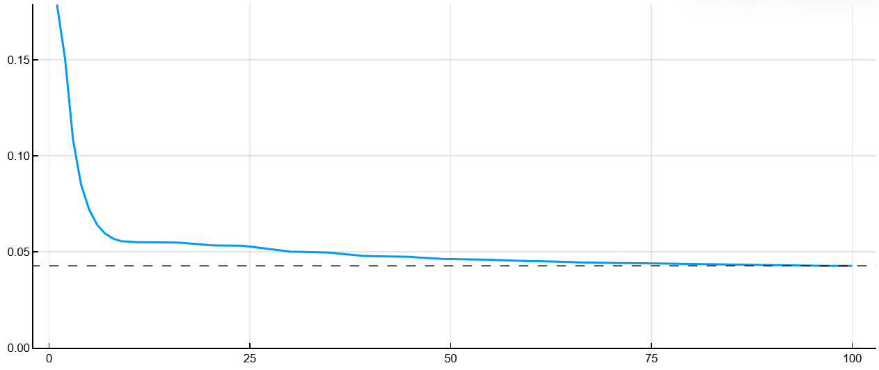
r,u,k,eEvol=rlevinson(ar,eFinal)Let’s plot the prediction errors. Add a horizontal line for the power of the final error. The error decreases with increasing filter order until the power of the final error is reached.
Let’s estimate the spectral power density (SPM) for orders of magnitude 1, 5, 25, 50 and 100. Let’s estimate the SPM for the initial autoregressive parameters.
N = [1, 5, 25, 50, 100]
nFFT = 8096
psdARpred = zeros(nFFT, 5)


for idx in 1:length(N)
    order = N[idx]
    ARpred = reverse(u[:, order], dims=1)
    psdARpred[:, idx] = 1 ./ abs.(fft(ARpred, nFFT)).^2
end


psdAR = 1 ./ abs.(fft(ar, nFFT)).^2
Let’s build a graph of SPM estimates. The SPM estimates for predictive filters gradually approach the initial autoregression parameters as the filter order increases.
F = (0:1/nFFT:1/2-1/nFFT) * Fs
pow2db(x) = 10 * log10.(x)

plot(F, pow2db.(psdARpred[1:end÷2, :]),
     xlabel = "Frequency (Hz)",
     ylabel = "Power (dB/Hz)",
     grid = true,
     legend = :best,
     xlims = (35, 70))


plot!(F, pow2db.(psdAR[1:end÷2]),
      linestyle = :dash,
      linecolor = :black,
      label = "Original AR")

order_labels = ["Order = $n" for n in N]

push!(order_labels, "Original AR")


plot!(serieslegend = order_labels)

display(current())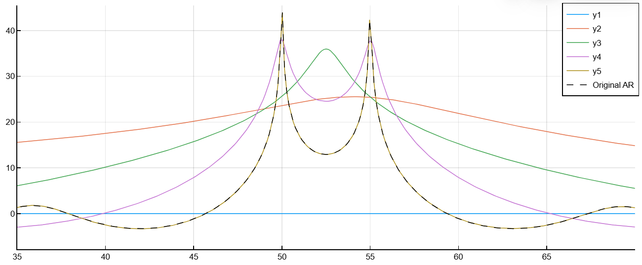
Algorithms
Levinson—Durbin inverse recursion implements a step-by-step algorithm for solving a symmetric system of linear Toeplitz equations.
where , , and the symbol denotes a complex conjugation.
In linear prediction applications:
-
Vector It is an autocorrelation sequence of input data for a predictive filter, where — element with zero delay. The Greenhouse Matrix — this is an autocorrelation matrix:
-
Vector it represents the coefficients of the predictive filter polynomial in descending order of degrees .
-
Scalar value indicates the order of the predictive filter.
The figure shows a typical filter of this type, where — optimal linear predictor, — input signal, — the predicted signal, and — prediction error signal. Variance of the prediction error — the scalar power of the prediction error.

Function rlevinson solves this system of equations to calculate the autocorrelation sequence r, having a vector a with the coefficients of the predictive filter. The filter must be minimum-phase in order to generate a valid autocorrelation sequence. Scalar eFinal represents the power of the final prediction error and it tends to be the target error of evaluating the Levinson—Durbin recursion, which the function implements. rlevinson.
To get the output data u, k and eEvolution function rlevinson it also performs decomposition inverse autocorrelation matrix . This decomposition resolves the matrices and and it allows you to efficiently calculate the inverse autocorrelation matrix. :
Output argument u returns the matrix . This matrix contains the recursive polynomials of the predictive filter from each iteration of the Levinson—Durbin inverse recursion:
Each vector contains the recursive coefficients of the polynomial, where — -th coefficient of the predictive filter polynomial -th order (i.e., -the th step of recursion). For example, the coefficients of the predictive filter polynomial The -th order can be obtained as , where a5 = u[5:−1:1, 5], and this vector is a polynomial . Therefore, -th column contains a vector of coefficients of the input polynomial a, which can be obtained using (u[p+1:−1:1, p+1])'.
Output argument k returns a column vector with reflection coefficients that are conjugate to the off-diagonal elements in the first row. . In other words, k returns as (u[1, 2:end])':
Output argument eEvolution returns a vector string with recursive prediction errors obtained from the diagonal of the matrix , except for the first element:
Each element enumerates the recursive predictions of the predictive filter polynomial -th order (i.e., -th step in recursion). For example, the prediction error of the predictive filter polynomial The -th order can be obtained as e5 = eEvolution(4) and this is a prediction error when using a polynomial as a predictive filter.
-
The first element on the diagonal , , coincides with the first element of the autocorrelation sequence , .
-
-th element on the diagonal , , is also the last element in
eEvolution— coincides with the power of the final prediction erroreFinal.