levinson
Levinson—Durbin recursion.
| Library |
|
Arguments
Input arguments
# n is the order of the model
+
length(r)−1 (by default) | a positive integer scalar
Details
The order of the model, given as a positive integer scalar.
| Data types |
|
Output arguments
# a — coefficients of the linear autoregression process
+
vector string | the matrix
Examples
Coefficients of the autoregression process
Details
We will generate the coefficients of the autoregressive process given by the expression
import EngeeDSP.Functions: randn,filter,xcorr,levinson

a = [1 0.1 -0.8 -0.27]
Let’s generate an implementation of the process by filtering out white noise with variance. 0.4.
v = 0.4
w = sqrt(v)*randn(15000,1)
x = filter(1,a,w)
Let’s evaluate the correlation function. Let’s discard the correlation values for negative lag intervals. We use Levinson—Durbin recursion to estimate the coefficients of the model. Let’s make sure that the prediction error corresponds to the variance of the input data.
r, lg = xcorr(x,"biased")
r = r[lg[:] .>= 0]
ar,e,k = levinson(r,numel(a)-1)
println("ar: ", ar)
println("e: ", e)
ar: [1.0 0.09735638301626465 -0.7977574280493284 -0.2697747348725144]
e: 0.39925318400516796Let’s estimate the reflection coefficients for the model 16- th order. Let’s make sure that the only reflection coefficients that lie outside the 95% of confidence bounds correspond to the correct order of the model.
ar,e,k = levinson(r,16)

stem(1:length(k[:]), k[:],
     marker=:circle,
     markercolor=:blue,
     linecolor=:blue)

conf = sqrt(2) * erfinv(0.95) / sqrt(15000)
x_limits = xlims()

X = [x_limits[1], x_limits[2]]
Y1 = [conf, conf]
Y2 = [-conf, -conf]

plot!(X, Y1, linestyle=:dash, color=:red, label="")
plot!(X, Y2, linestyle=:dash, color=:red, label="")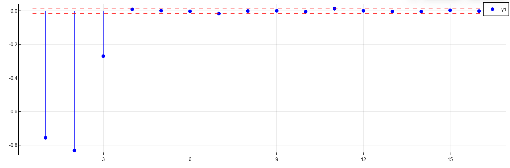
Prediction errors for multiple implementations
Details
We will generate the coefficients of the autoregressive process given by the expression
import EngeeDSP.Functions: randn,filter,xcorr,levinson

a = [1 0.1 -0.8 -0.27]
We will generate five process implementations by filtering out white noise with different variances.
nr = 5
v = rand(1,nr)
1×5 Matrix{Float64}:
0.264731 0.244259 0.401966 0.184345 0.070915w = sqrt.(v[:])' .* randn(15000, nr)
x = filter(1,a,w)Let’s evaluate the correlation function. Let’s discard the cross-correlation terms and correlation values for negative lag intervals. We will use Levinson—Durbin recursion to estimate the prediction errors for the correct model order and make sure that the prediction errors correspond to the variances of the input noise signals.
r, lg = xcorr(x,"biased")

ar,e,k = levinson(r[lg[:] .>= 0,1:nr+1:end],numel(a)-1)

println("e: ", e)
e: [0.26082618781928835; 0.24091448115262645; 0.40999877779431343; 0.18019545485810384; 0.07090107526341564;;]Algorithms
Levinson—Durbin recursion is an algorithm for finding an all—pole IIR filter with a given deterministic autocorrelation sequence. It finds applications in filter design, coding, and spectral analysis. The filter that uses levinson, is a minimum phase filter.
Function levinson solves a symmetric system of linear equations Greenhouse:
where r is the input autocorrelation vector, and denotes a complex conjugation . The input vector r It is usually a vector of autocorrelation coefficients, where is the lag interval 0 is the first element .
If r if there is no correct autocorrelation sequence, then the function levinson It can return values NaN even if a solution exists.
|
The algorithm requires operations and is therefore much more efficient than the operator \ for large values n. However, the function levinson uses \ for low orders, to ensure the fastest possible execution.